38 Wyniki
Wyświetl wyniki:
Sortuj według:
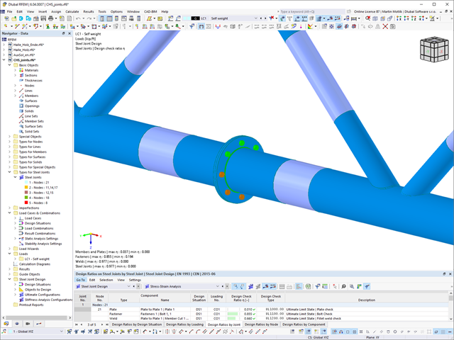
W rozszerzeniu Połączenia stalowe można łączyć profile zamknięte o przekroju okrągłym za pomocą spoin.
Profile okrągłe można łączyć ze sobą lub z płaskimi elementami konstrukcyjnymi. Spoiną można również łączyć pachwiny przekrojów znormalizowanych i cienkościennych.
Przejdź do filmu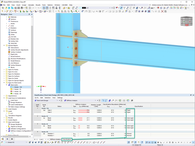
W rozszerzeniu Połączenia stalowe można klasyfikować sztywności połączeń.
Oprócz sztywności początkowej w tabeli wyświetlane są również wartości graniczne dla połączeń przegubowych i sztywnych dla wybranych sił wewnętrznych N, My i/lub Mz. Uzyskana klasyfikacja jest następnie wyświetlana w tabeli jako „przegubowa”, „półsztywna” i „sztywna”.
Przejdź do filmu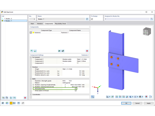
W rozszerzeniu „Połączenia stalowe” można uwzględnić naprężenie wstępne śrub w obliczeniach dla wszystkich komponentów. Sprężenie można łatwo aktywować za pomocą pola wyboru w parametrach śruby i ma ono wpływ zarówno na analizę naprężeniowo-odkształceniową, jak i na analizę sztywności.
Śruby sprężone to specjalne śruby stosowane w konstrukcjach stalowych w celu wygenerowania dużej siły zaciskowej między połączonymi elementami konstrukcyjnymi. Ta siła docisku powoduje tarcie między elementami konstrukcyjnymi, co umożliwia przenoszenie sił.
Funkcjonalność
Śruby sprężane są dokręcane z określonym momentem, co powoduje ich rozciąganie i powstawanie siły rozciągającej. Ta siła rozciągająca jest przenoszona na połączone elementy i prowadzi do powstania dużej siły mocującej. Siła zaciskowa zapobiega poluzowaniu połączenia i zapewnia niezawodne przenoszenie siły.
Zalety
- Wysoka nośność: Śruby wstępnie rozciągane mogą przenosić duże siły.
- Niskie odkształcenie: Minimalizują odkształcenie połączenia.
- Wytrzymałość zmęczeniowa: Są odporne na zmęczenie.
- Łatwość montażu: Są one stosunkowo łatwe w montażu i demontażu.
Analiza i wymiarowanie
Obliczenia śrub sprężanych są przeprowadzane w RFEM z wykorzystaniem modelu analitycznego ES wygenerowanego przez rozszerzenie "Połączenia stalowe". Uwzględnia ona siłę zwarcia, tarcie między elementami konstrukcyjnymi, wytrzymałość śrub na ścinanie oraz nośność elementów konstrukcyjnych. Wymiarowanie odbywa się zgodnie z DIN EN 1993-1-8 (Eurokod 3) lub amerykańską normą ANSI/AISC 360-16. Utworzony model analityczny wraz z wynikami można zapisać i wykorzystać jako niezależny model w programie RFEM.
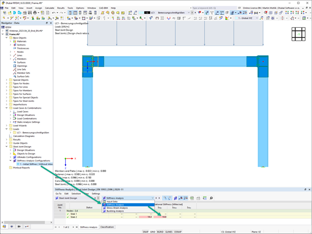
Sztywność początkowa Sj,ini jest parametrem decydującym o ocenie, czy połączenie można scharakteryzować jako sztywne, niesztywne czy przegubowe.
W rozszerzeniu „Połączenia stalowe” można obliczyć początkowe sztywności Sj,ini zgodnie z Eurokodem (EN 1993-1-8 sekcja 5.2.2) i AISC (AISC 360-16 Cl. E3.4) w odniesieniu do sił wewnętrznych N, My i/lub Mz.
Opcjonalne automatyczne przenoszenie sztywności początkowych umożliwia bezpośrednie przenoszenie sztywności przegubowych na końcach prętów w programie RFEM. Następnie cała konstrukcja jest ponownie obliczana, a wynikające z niej siły wewnętrzne są automatycznie uwzględniane jako obciążenia w obliczeniach i wymiarowaniu modeli połączeń.
Ten zautomatyzowany proces iteracji eliminuje konieczność ręcznego eksportu i importu danych, zmniejszając ilość pracy i minimalizując potencjalne źródła błędów.
Film wyjaśniający: Obliczanie sztywności początkowej Sj,ini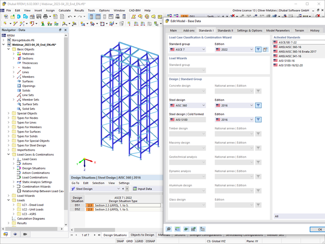
Wymiarowanie prętów stalowych formowanych na zimno zgodnie z AISI S100-16/CSA S136-16 jest dostępne w RFEM 6. Dostęp do obliczeń można uzyskać, wybierając normy „AISC 360” lub „CSA S16” w rozszerzeniu Projektowanie konstrukcji stalowych. Następnie dla obliczeń elementów formowanych na zimno automatycznie wybierane jest „AISI S100” lub „CSA S136”.
Do obliczania sprężystego obciążenia wyboczeniowego pręta program RFEM stosuje metodę DSM. Bezpośrednia metoda wytrzymałości oferuje dwa typy rozwiązań, numeryczne (metoda pasm skończonych) i analityczne (specyfikacja). Krzywą charakterystyczną (sygnaturę) FSM i kształty wyboczenia można wyświetlić w oknie dialogowym Przekroje.
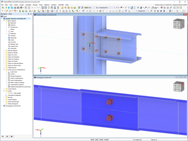
Rozszerzenie Połączenia stalowe umożliwia wymiarowanie połączeń prętów o złożonych przekrojach. Ponadto można przeprowadzać obliczenia połączeń dla prawie wszystkich przekrojów cienkościennych z biblioteki programu RFEM.
Przejdź do filmu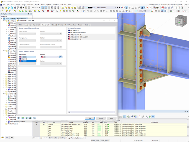
W rozszerzeniu Połączenia stalowe można wymiarować połączenia zgodnie z amerykańską normą ANSI/AISC 360-16. Zintegrowane zostały następujące metody obliczeń:
- Obliczenia współczynnika obciążenia i odporności (LRFD)
- Projektowanie dopuszczalnych naprężeń (ASD)
- 002567
- Ogólne informacje
- Projektowanie konstrukcji stalowych RFEM 6
- Projektowanie konstrukcji stalowych RSTAB 9
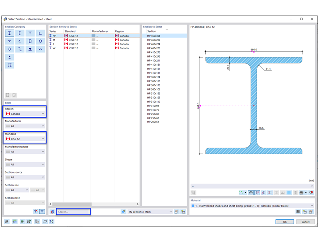
Nowe przekroje stalowe zgodnie z najnowszą instrukcją CISC (12 wydanie) są dostępne w programie RFEM 6. Przekroje są wymienione w bibliotece Znormalizowane. W filtrze należy wybrać region „Kanada”, a normę „CISC 12”. Alternatywnie nazwę przekroju można wprowadzić bezpośrednio w polu wyszukiwania znajdującym się w dolnej części okna dialogowego.

- 002133
- Ogólne informacje
- Projektowanie konstrukcji drewnianych RFEM 6
- Projektowanie konstrukcji drewnianych RSTAB 9
- Szeroki wybór przekrojów, takich jak przekroje prostokątne, kwadratowe, teowe, okrągłe, złożone, nieregularne przekroje parametryczne i wiele innych (przydatność do obliczeń zależy od wybranej normy)
- Wymiarowanie drewna klejonego krzyżowo (CLT)
- Wymiarowanie materiałów drewnopochodnych i drewna klejonego warstwowo zgodnie z EC 5
- Wymiarowanie prętów o zmiennym przekroju (metoda zgodna z normą)
- Możliwe jest dostosowanie istotnych współczynników obliczeniowych i parametrów normowych
- Elastyczność dzięki szczegółowym opcjom ustawień dla podstawy i zakresu obliczeń
- Szybkie i przejrzyste wyświetlanie wyników dla globalnej oceny ich rozkładu na konstrukcji po zakończeniu obliczeń
- Szczegółowe wyniki obliczeń i niezbędne wzory (jasna i łatwa do zweryfikowania ścieżka wyników)
- Przejrzyste zestawienie wyników w formie numerycznej w stosownych oknach oraz możliwość ich graficznego przedstawienia na konstrukcji
- Integracja wyników z protokołem wydruku programu RFEM/RSTAB
- 002372
- Ogólne informacje
- Projektowanie konstrukcji drewnianych RFEM 6
- Projektowanie konstrukcji drewnianych RSTAB 9
- Dowolna definicja czasu zwęglania
- W przypadku konstrukcji powierzchniowych (drewno klejone krzyżowo) można obliczyć z przyczepnością lub bez
- Bezpłatna, zdefiniowana przez użytkownika specyfikacja parametrów pożaru
- Uwzględnienie różnych długości efektywnych do obliczania odporności ogniowej
- Opcjonalne obliczenia dla 'ściskania w poprzek włókien'
- Zintegrowane z RFEM/RSTAB graficzne wyświetlanie wyników, np. B. Stopień wykorzystania
- Pełna integracja wyników z protokołem wydruku programu RFEM/RSTAB
- 002385
- Ogólne informacje
- Projektowanie konstrukcji drewnianych RFEM 6
- Projektowanie konstrukcji drewnianych RSTAB 9
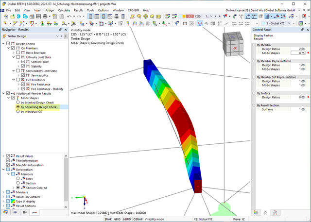
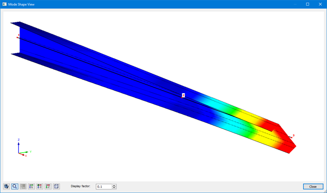
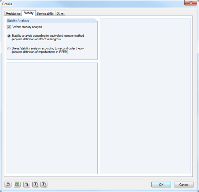
Czy do określenia współczynnika obciążenia krytycznego w ramach analizy stateczności użyto solwera wartości własnych rozszerzenia? W takim przypadku można wyświetlić decydujący kształt drgań własnych projektowanego obiektu. W tym miejscu dostępny jest solwer wartości własnych do analizy zwichrzenia, w zależności od zastosowanej normy obliczeniowej.
- 002387
- Obliczenia
- Projektowanie konstrukcji drewnianych RFEM 6
- Projektowanie konstrukcji drewnianych RSTAB 9
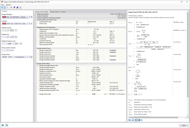
Jeśli projekt się powiedzie, nadejdzie czas. Ponieważ program wykonuje za Ciebie wiele procesów. Przeprowadzone kontrole obliczeń są na przykład wyświetlane w tabeli. Tutaj wyświetlane są wszystkie szczegóły wyników. Dzięki przejrzyście przedstawionym wzorom obliczeniowym wyniki są bezproblemowe i zrozumiałe. Nie ma tu efektu "czarnej skrzynki".
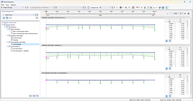
Obliczenia są przeprowadzane we wszystkich decydujących miejscach prętów i przedstawiane graficznie w postaci wykresu wyników. Ponadto w wynikach dostępne są szczegółowe grafiki, takie jak rozkład naprężeń w przekroju lub decydujący kształt postaci drgań.
Wszystkie dane wejściowe i wyniki są częścią protokołu wydruku programu RFEM/RSTAB. Zawartość protokołu i jego zakres można wybrać specjalnie dla poszczególnych warunków projektowych.
- 002089
- Ogólne informacje
- Skręcanie skrępowane (7 stopni swobody) RFEM 6
- Skręcanie skrępowane (7 stopni swobody) RSTAB 9
- Uwzględnienie 7 lokalnych kierunków deformacji (ux , uy, uz, φx, φy, φz, ω ) lub 8 sił wewnętrznych (N , Vu, Vv, Mt, pri, Mt, s, Mu, Mv, Mω ) przy obliczaniu elementów prętowych
- Możliwość stosowania w połączeniu z analizą statyczno-wytrzymałościową według teorii II rzędu, i analiza dużych deformacji (można również uwzględnić imperfekcje)
- W połączeniu z rozszerzeniem Analiza stateczności umożliwia definiowanie współczynników obciążenia krytycznego i kształtów drgań dla problemów stateczności, takich jak wyboczenie skrętne i zwichrzenie
- Uwzględnianie blach czołowych i usztywnień poprzecznych jako sprężystości skrępowanej podczas obliczania przekrojów dwuteowych z automatycznym określaniem i wyświetlaniem graficznym sztywności sprężystości deplanacyjnej
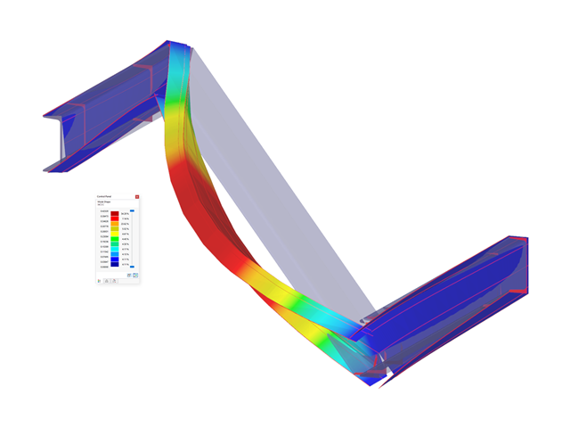
- Graficzne przedstawienie deplanacji przekroju prętów w stanie odkształcenia
- Pełna integracja z RFEM i RSTAB

- 002090
- Ogólne informacje
- Skręcanie skrępowane (7 stopni swobody) RFEM 6
- Skręcanie skrępowane (7 stopni swobody) RSTAB 9
Obliczenia skręcania skrępowanego można przeprowadzić dla całego układu. Uwzględniasz zatem dodatkową wartość 7 stopnia swobody w obliczeniach pręta. Sztywności połączonych elementów konstrukcyjnych są uwzględniane automatycznie. Oznacza to, że nie ma potrzeby' definiowania równoważnych sztywności sprężystych ani warunków podparcia dla układu odłączanego.
Następnie można wykorzystać siły wewnętrzne z obliczeń ze skręcaniem skrępowanym w rozszerzeniu do obliczeń. W zależności od materiału i wybranej normy należy uwzględnić bimoment wyboczeniowy i drugorzędny moment skręcający. Typowym zastosowaniem jest analiza stateczności według teorii drugiego rzędu z wykorzystaniem imperfekcji w konstrukcjach stalowych.
Czy wiecie, że...? Zastosowanie nie ogranicza się do przekrojów stalowych cienkościennych. Pozwala to na przykład na przeprowadzenie obliczeń idealnego momentu krytycznego dla belek o przekrojach z drewna litego.
- 002401
- Ogólne informacje
- Skręcanie skrępowane (7 stopni swobody) RFEM 6
- Skręcanie skrępowane (7 stopni swobody) RSTAB 9
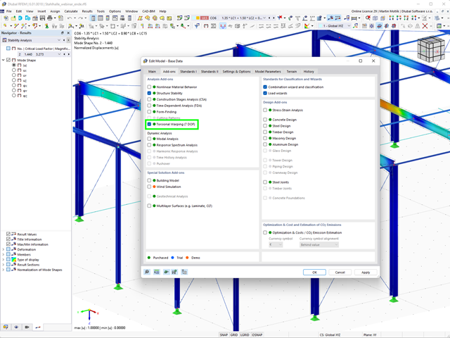
- Funkcję skręcania skrępowanego można aktywować lub dezaktywować w zakładce Rozszerzenia w Danych podstawowych modelu.
- Po aktywowaniu rozszerzenia interfejs użytkownika w programie RFEM zostaje rozszerzony o nowe wpisy w nawigatorze, tabelach i oknach dialogowych.
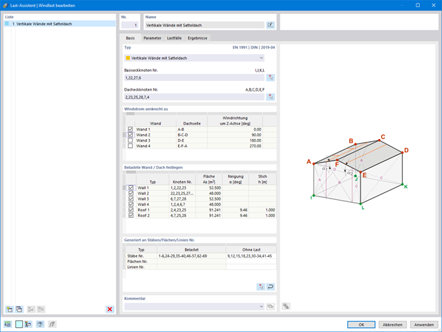
Obciążenia wiatrem również nie stanowią problemu w obliczeniach. Obciążenia wiatrem mogą być generowane automatycznie jako obciążenia prętowe lub obciążenia powierzchniowe (RFEM) na następujących elementach konstrukcyjnych:
- Ściany pionowe
- Dachy płaskie
- Dachy jednospadowe
- Dachy dwuspadowe/korytowe
- Ściany pionowe z dachem dwuspadowym
- Ściany pionowe z dachem płaskim/jednospadowym
Dostępne są następujące normy:
-
 EN 1991-1-4 (wraz z załącznikami krajowymi)
 -
 ASCE 7
 -
 NBC
NBC -
 CTE DB-SE-AE
 -
 GB 50009
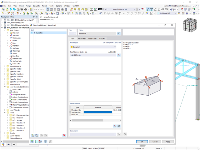
Czy Twoje konstrukcje również muszą wytrzymać opady śniegu? Za pomocą Kreatora obciążeń śniegiem można generować obciążenia śniegiem jako obciążenia prętowe lub powierzchniowe.
Dostępne są poniższe normy:
-
EN 1991-1-3 (wraz z załącznikami krajowymi)
-
ASCE 7
-
NBC
-
 SIA 261
 -
CTE DB-SE-AE
-
GB 50009
-
 IS 875
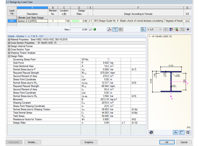
Dzięki zintegrowanemu rozszerzeniu modułu RF-/STEEL Warping Torsion, możliwe jest przeprowadzenie obliczeń zgodnie z Design Guide 9 w RF-/STEEL AISC.
Obliczenia są przeprowadzane z 7 stopniami swobody zgodnie z teorią skręcania skrępowanego i umożliwiają realistyczne obliczenia stateczności z uwzględnieniem skręcania.
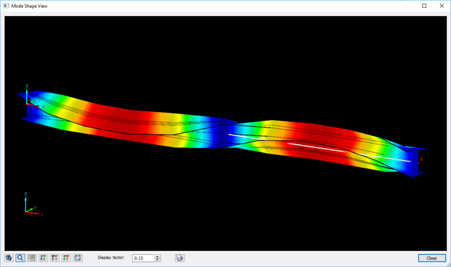
Definiowanie krytycznego momentu wyboczeniowego odbywa się w module RF-/STEEL AISC za pomocą solwera wartości własnych, który umożliwia dokładne określenie krytycznego obciążenia wyboczeniowego.
Solwer wartości własnych pokazuje okno z grafiką wartości własnych, które umożliwia sprawdzenie warunków brzegowych.
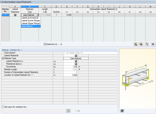
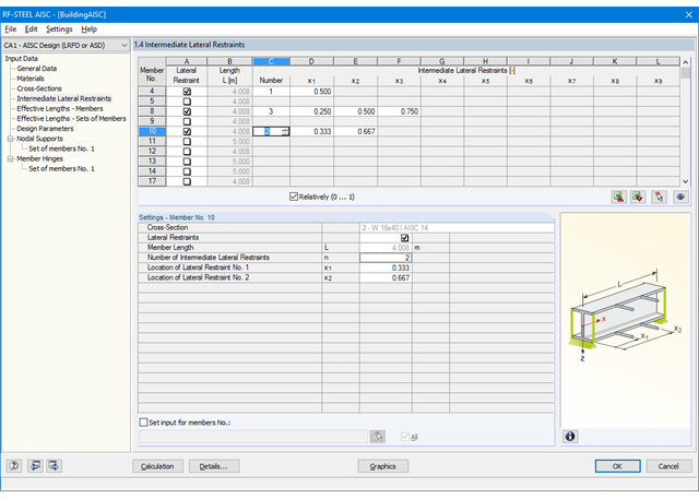
W programie STEEL AISC możliwe jest uwzględnienie pośrednich podpór bocznych w dowolnym miejscu. Na przykład, możliwa jest stabilizacja tylko górnej półki.
Ponadto można przypisać boczne podpory pośrednie zdefiniowane przez użytkownika; na przykład pojedyncze sprężyny obrotowe i sprężyny translacyjne w dowolnym miejscu przekroju.
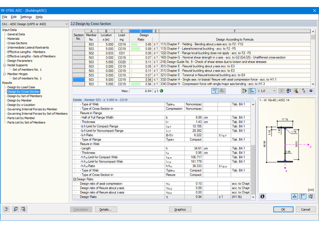
Pierwsze okno wyników pokazuje maksymalne stopnie wykorzystania wraz z odpowiednim wykorzystaniem dla każdego obliczanego przypadku obciążenia, kombinacji obciążeń lub kombinacji wyników.
W pozostałych oknach wyników wyświetlane są wszystkie szczegółowe wyniki posortowane według określonego tematu w rozwijanych menu. Wszystkie wyniki pośrednie wzdłuż prętów można wyświetlić w dowolnym miejscu. W ten sposób można łatwo prześledzić, w jaki sposób moduł przeprowadził poszczególne obliczenia.
Pełne dane modułu stanowią część protokołu wydruku programu RFEM/RSTAB. Zawartość i zakres protokołu można wybrać indywidualnie dla poszczególnych obliczeń.
Najpierw należy zdecydować, czy obliczenia mają być przeprowadzone zgodnie z ASD czy LRFD. Następnie można wprowadzić przypadki obciążeń, kombinacje obciążeń i kombinacje wyników, które mają zostać obliczone. Kombinacje obciążeń zgodnie z ASCE 7 można generować ręcznie lub automatycznie w programie RFEM/RSTAB.
W kolejnych krokach można dostosować wstępne ustawienia bocznych podpór pośrednich, długości efektywnych i innych parametrów obliczeniowych specyficznych dla normy, takich jak współczynnik modyfikacjiCb dla zwichrzenia lub współczynnika niezrealizowanego nośności. W przypadku prętów ciągłych można zdefiniować indywidualne warunki podparcia i mimośrody każdego węzła pośredniego pojedynczych prętów. Specjalne narzędzie dla analizy MES, które działa w tle, określa obciążenia krytyczne oraz momenty wymagane dla analizy stateczności.
W połączeniu z programem RFEM/RSTAB, możliwe jest zastosowanie metody analizy bezpośredniej z uwzględnieniem wpływu obliczeń ogólnych zgodnie z teorią drugiego rzędu. W ten sposób unika się stosowania specjalnych współczynników powiększenia.
- Wymiarowanie prętów i zbiorów prętów dla rozciągania, ściskania, zginania, ścinania, kombinacji sił wewnętrznych i skręcania
- Analiza stateczności dla wyboczenia i zwichrzenia
- Automatyczne określanie krytycznych obciążeń wyboczeniowych i krytycznych momentów wyboczeniowych dla ogólnych obciążeń i warunków podparcia za pomocą specjalnego programu MES (analizy wartości własnych) zintegrowanego w module
- Alternatywne obliczenia analityczne krytycznego momentu wyboczeniowego dla sytuacji standardowych
- Możliwość zastosowania oddzielnych podpór bocznych do belek i prętów ciągłych
- Automatyczna klasyfikacja przekrojów (zwarty, niezwarty, smukły)
- Obliczenia w stanie granicznym użytkowalności (ugięcie)
- Optymalizacja przekroju
- Szeroki wybór dostępnych przekrojów, takich jak np. dwuteowniki walcowane; ceowniki; teowniki; kątowniki; profile zamknięte prostokątne i okrągłe; pręty okrągłe; przekroje symetryczne i niesymetryczne, parametryczne przekroje dwuteowe, teowe, kątowniki; podwójne kątowniki
- Przejrzyste okna wprowadzania i wyników
- Szczegółowa dokumentacja wyników wraz z odniesieniami do równań obliczeniowych z zastosowanej normy
- Różne opcje filtrowania i sortowania wyników, w tym listy wyników według prętów, przekrojów i położenia x, przypadków obciążeń, kombinacji obciążeń i kombinacji wyników
- Tabela wyników dla smukłości pręta i głównych sił wewnętrznych
- Wykaz części z parametrami masy i masy
- Pełna integracja z programem RFEM/RSTAB
- Jednostki metryczne i anglosaskie
- Stosuje się do prętów zdefiniowanych jako zbiory prętów
- Oddzielny solwer uwzględniający 7 kierunków deformacji (ux , uy, uz, φx, φy, φz, ω ) lub 8 sił wewnętrznych (N, Vu, Vv, Mt, pri, Mt, s, Mu, Mv,M )
- Projektowanie nieliniowe według analizy drugiego rzędu
- Wprowadzanie imperfekcji
- Obliczanie współczynników obciążenia krytycznego i postaci wyboczenia oraz ich wizualizacja (wraz z skręcaniem skrępowanym)
- Integracja z wymiarowaniem prętów w modułach dodatkowych RF-/STEEL AISC i RF-/STEEL EC3
- Dostępne dla wszystkich przekrojów stalowych cienkościennych
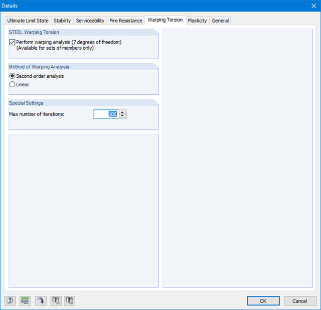
Ponieważ moduł RF-/STEEL Warping Torsion jest w pełni zintegrowany z modułami RF-/STEEL AISC i RF‑/STEEL EC3, dane są wprowadzane w taki sam sposób, jak w przypadku obliczeń w tych modułach. W oknie dialogowym Szczegóły, zakładka Skręcanie skrępowane (patrz rysunek po prawej stronie), konieczne jest tylko zaznaczenie opcji "Przeprowadzić analizę skręcania skrępowanego". W tym oknie dialogowym można również zdefiniować maksymalną liczbę iteracji.
Analiza skręcania skrępowanego jest przeprowadzana dla zbiorów prętów w modułach RF-/STEEL AISC i RF-/STEEL EC3. Można dla nich zdefiniować warunki brzegowe, takie jak podpory węzłowe lub zwolnienia na końcach prętów.
Możliwe jest również określenie imperfekcji do obliczeń nieliniowych.
Wyniki analizy skręcania skrępowanego są wyświetlane w modułach RF-/STEEL AISC i RF-/STEEL EC3 w zwykły sposób. Odpowiednie okna wyników zawierają między innymi wartości krytycznego skręcania i skręcania, siły wewnętrzne oraz podsumowanie obliczeń.
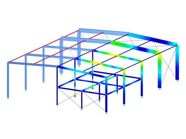
Graficzne przedstawienie postaci drgań (wraz z deplanacją) umożliwia realistyczną ocenę zachowania się wyboczenia.
Obliczenia nośności przekroju obejmują analizę rozciągania i ściskania wzdłuż włókien, zginania, zginania i rozciągania/ściskania oraz wytrzymałości na ścinanie.
Elementy konstrukcyjne z możliwością wyboczenia i zwichrzenia są analizowane według metody pręta zastępczego i uwzględniane są systematyczne ściskanie osiowe, zginanie z lub bez siły ściskającej oraz zginanie i rozciąganie. Ugięcie wewnętrznych przęseł i wsporników jest porównywane z maksymalnym dopuszczalnym ugięciem.
Oddzielne przypadki obliczeniowe umożliwiają elastyczną analizę stateczności prętów, zbiorów prętów i obciążeń.
Parametry istotne dla obliczeń, takie jak analiza stateczności, czas trwania obciążenia w warunkach pożaru, smukłość prętów i ugięcie graniczne, można dostosowywać zgodnie z potrzebami.
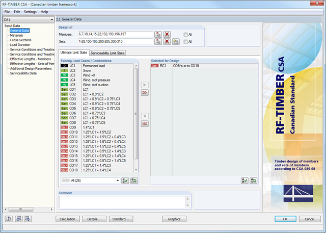
Po otwarciu modułu należy wybrać pręty/zbiory prętów, przypadki obciążeń, kombinacje obciążeń lub kombinacje wyników dla obliczeń stanu granicznego nośności i użytkowalności. Materiały z programu RFEM/RSTAB są wstępnie ustawione i można je dostosować w RF-/TIMBER CSA. Charakterystyki materiałowe zgodne z odpowiednimi normami zapisane są w bibliotece.
Podczas sprawdzania przekrojów można określić, czy uwzględniany jest przekrój wybrany w programie RFEM/RSTAB, czy przekrój zmodyfikowany. Następnie można zdefiniować klasy trwania obciążenia, warunki wilgotnościowe oraz obróbkę drewna.
Do analizy deformacji wymagane są długości referencyjne odpowiednich prętów i zbiorów prętów. Ponadto można zdefiniować określony kierunek ugięcia, wygięcie wstępne i typ belki.
W przypadku obliczeń odporności ogniowej można zdefiniować strony zwęglenia pręta lub zbioru prętów.
- Wymiarowanie prętów na rozciąganie, ściskanie, zginanie, ścinanie i kombinację sił wewnętrznych
- Analiza stateczności dla wyboczenia i zwichrzenia według metody pręta zastępczego lub analizy drugiego rzędu
- Analiza stateczności dla wyboczenia i zwichrzenia według metody pręta zastępczego lub teorii drugiego rzędu
- Dowolna konfiguracja czasu i prędkości zwęglania oraz dowolny wybór stron zwęglania do obliczeń odporności ogniowej
- Swobodne ustalenie szybkości zwęglania, czasu oraz stron narażonych na działanie ognia przy obliczaniu odporności ogniowej
- Kanadyjska baza materiałów i biblioteka przekrojów
- Zdefiniowane przez użytkownika wprowadzanie przekrojów prostokątnych i okrągłych
- Automatyczna optymalizacja przekrojów
- Możliwość importowania długości wyboczeniowych z modułu dodatkowego RF-STABILITY/RSBUCK
- Szczegółowa dokumentacja wyników wraz z odniesieniami do równań obliczeniowych z zastosowanej normy
- Różne opcje filtrowania i sortowania wyników
- Uwzględnienie wpływu warunków wilgotności drewna
- Wizualizacja kryterium obliczeniowego na modelu w programie RFEM/RSTAB
- Eksport danych do MS Excel
- Jednostki metryczne i imperialne
Po zakończeniu obliczeń wyniki wyświetlane są w przejrzyście ułożonych tabelach. Aby obliczenia były bardziej przejrzyste, można uwzględnić wszystkie wartości pośrednie (np. decydujące siły wewnętrzne, współczynniki korekcyjne itp.). Wyniki są posortowane według przypadków obciążenia, przekrojów, zbiorów prętów i prętów. Jeżeli analiza nie powiedzie się, przekroje, których to dotyczy, można zmodyfikować w procesie optymalizacji.
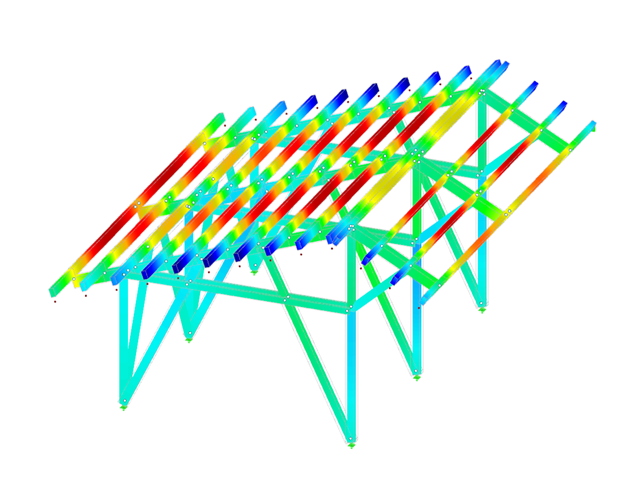
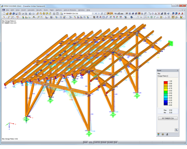
Stopień wykorzystania jest przedstawiony na modelu w programie RFEM/RSTAB za pomocą kolorów. W ten sposób można szybko rozpoznać obszary krytyczne lub przewymiarowane. Dokładną ocenę zapewniają wykresy wyników wyświetlane na pręcie lub zbiorze prętów.
Oprócz danych wejściowych i wyników, w tym szczegółowych informacji dotyczących obliczeń, wyświetlanych w tabelach, do protokołu wydruku można dodać wszystkie grafiki. W ten sposób dokumentacja jest przejrzysta i zrozumiała. Użytkownik może dostosować zawartość protokołu i żądany zakres wyników dla poszczególnych warunków projektowych.