


The design of a floor slab made of steel fiber-reinforced concrete consists of the ultimate limit state design and the serviceability limit state design. The procedure for performing the ultimate limit state design has already been explained in a previous Technical Article.
The serviceability limit state design is now performed for the floor slab discussed in the previous article. This article shows how to perform the corresponding design for the SLS by means of the iteratively determined FEA results.
Entering Topology and Loads
The plate geometry and imposed loads are transferred from the ultimate limit state design (see the technical article mentioned above).
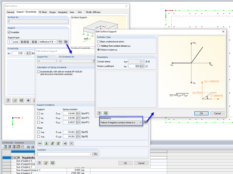
For the serviceability limit state design, the positive effects from shrinkage must also be taken into account. When shrinking, the floor slab wants to contract. Due to the interconnection or friction of the floor slab on the subsoil, tensile stresses occur which have to be considered. The base plate is embedded on the following layer structure (from top to bottom): Base plate, foil as a separating layer, perimeter insulation, bottom concrete layer, soil. According to [3], Table 4.19, a friction coefficient μ0 of 0.8 is recommended for this layer structure. For the design value μ0,d, the authors of [3] recommend a partial safety factor of γR = 1.25.
In RFEM, the friction coefficient μ0,d can be defined as the nonlinearity of the surface elastic foundation. Image 02 shows the setting option in the program.
In the case of industrial floor slabs, the vertical load is of great importance for the formation of the positive action due to shrinkage strain. Before the racking loads are applied and the stored goods are placed, only the self-weight of the floor slab is available. As a result, the friction resistance of the bottom floor slab is relatively small. The tensile force Nctd resulting from the friction (in relation to a 1-meter-wide strip) in the base plate is determined as follows.
|
Nctd |
Design value to determine the tensile stress in the floor slab when the friction force is reached |
|
μ0,d |
Design value of friction |
|
σ0 |
Contact Pressure |
|
L |
Length of the base plate for the displacement on the soil |
σ0 = 0.19 m ⋅ 1.0 m ⋅ 25 kN/m² = 4.35 kN/m² (self-weight of the slab)
Nctd = 1.0 ⋅ 4.75 kN/m² ⋅ 24.40 m/2 = 57.95 kN/m
The maximum resulting tensile stress σct,d resulting from friction thus results in
σct,d = Nctd / Act = 57.95 kN/m / 0.19 m = 305 kN/m² = 0.305 MN/m² <f fctm,fl = 2.9 MN/m².
The concrete tensile stress resulting from friction under the self-weight of the floor slab is lower than the concrete tensile strength ffctm,fl. This allows the shrinkage strain to occur without cracking under the panel's dead load.
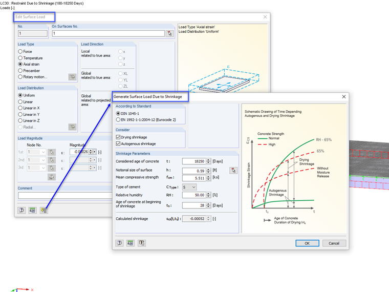
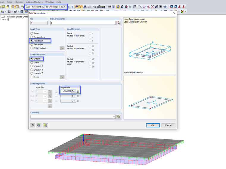
However, once the rack loads/support loads have been applied, the increased friction forces under the higher rack supports result in restraint forces that must be taken into account in the calculation. In this project, t = 180 days after concreting the base plate is assumed as the time at which the rack loads are applied. To calculate the shrinkage strain, ts = 7 days is used as the start of shrinkage and t = 18,250 days as the end of use. A relative humidity of 50% is also assumed. The shrinkage strain is applied as an external surface load by means of the axial strain load type. At this point, it should be noted that an auxiliary tool is built into the Surface Load dialog box, which makes it very easy to determine the shrinkage strain.

When applying the shrinkage strain, you must take into account that shrinkage up to the time t = 180 days does not cause any restraints in the plate. Therefore, only the positive shrinkage strain εcs,wk has to be applied for the design check at the time t = 18,250 days. This is calculated as the difference of the shrinkage strains at t = 18,250 and t = 180 days. No detailed calculation of the individual shrinkage strains is described in this article.
εcs,wk = εcs (18,250, 7) - εcs (180, 7) = -0.515‰ - (-0.258‰) = 0.257‰
The positive shrinkage strain is defined as an additional load and taken into account in the load combinatorics for the time t = 18,250 days.
For the serviceability limit state design, the "Quasi-permanent" design situation is required. The variable load for storage spaces is taken into account with the combination factor ψ2 = 0.8. These load combinations are used for stress checks and for limiting the crack width due to loading.
In order to consider the imposed action from shrinkage at the end of use (t = 18,250 days), the previously created load combinations are copied and the "Shrinkage" load case is added to the positive shrinkage strain εcs,wk. These load combinations are used later for the crack width analysis under load action with restraint.
Define Material Properties for Serviceability Limit State Design
Use the "Isotropic Damage 2D/3D" material model of the RF-MAT NL add-on module to display the material behavior of steel fiber-reinforced concrete in RFEM. We use C30/37 L1.2/L0.9 concrete as steel fiber-reinforced concrete in accordance with DIN EN 1992-1-1 [2] and the guideline by the German Committee for Reinforced Concrete (DAfStb) on steel fiber-reinforced concrete [1] with the two performance classes L1/L2 = L1.2/L0.9. For a nonlinear calculation, the parabolic curve according to 3.1.5 [2] must be used on the compression side of the stress-strain diagram. Image 05 shows the characteristic curve of the working line of the aforementioned steel fiber-reinforced concrete.
We have to use the characteristic stress-strain curve for the serviceability limit state. An Excel file is attached to this article as an input aid or tool for calculating the diagram points. You can transfer these diagram points to the RFEM input dialog box using the clipboard (see also the recommendations in the article about the ULS design).
Sserviceability Limit State Design
When performing the serviceability limit state design, it is necessary to design the maximum allowable:
- Limit stresses according to 7.2, DIN EN 1992-1-1 [2]
- Crack widths according to 7.3, DIN EN 1992-1-1 [2]
- Deformations according to 7.4, DIN EN 1992-1-1 [2]
After successful nonlinear calculation of the base plate, the strains and stresses on the top and bottom sides are evaluated and used for the individual design checks.
A) Design of Limit Stresses
The design of the maximum concrete compressive stress according to 7.2 (3) [2] is fulfilled if the maximum concrete compressive stress remains less than 0.45 ⋅ fck under quasi-permanent load action. For this purpose, the minimum stresses on the top and bottom sides are checked from the FEM calculation and compared to the limit value.
Top side:
Maximum compressive stress σ2- = | - 8.5 | N/mm² <0.45 ⋅ fck = 13.5 N/mm²
Bottom side:
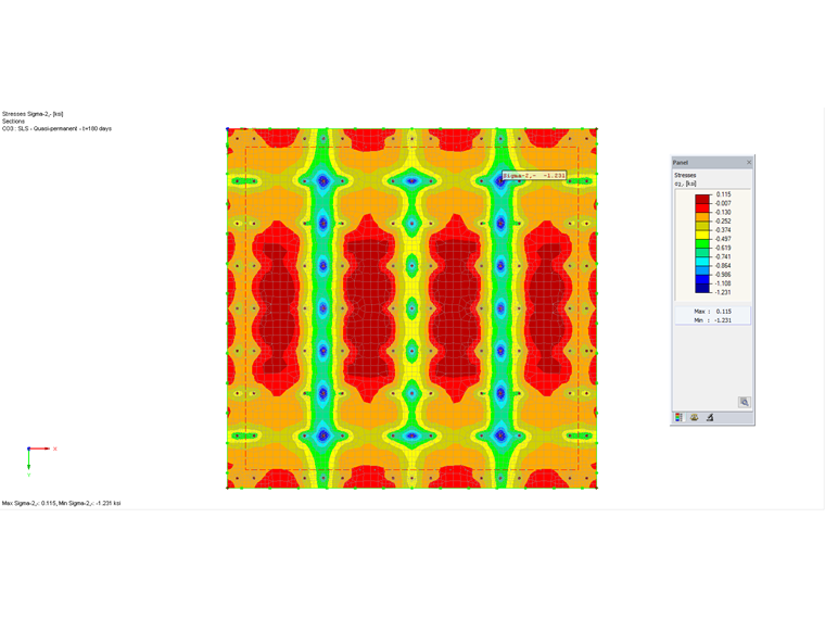
Maximum compressive stress σ2+ = | - 3.1 | N/mm² <0.45 ⋅ fck = 13.5 N/mm²
Image 06 shows the maximum compressive stress on the top side (-z) of the foundation plate.
Maintaining the maximum concrete compressive stress is successfully verified.
The design of the limitation of the maximum reinforcing steel stress according to 7.2. (4) and (5) [2] is not required here, as there is no rebar reinforcement.
B) Crack Width Analysis from Load Action
The crack width analysis is performed for the pure load action (at time t = 180 days) and with additional consideration of the restraint due to shrinkage at the end of use (t = 18,250 days). See also the explanations above regarding shrinkage.
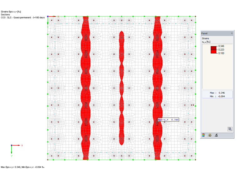
The existing crack width is determined on the basis of the quasi-permanent action combination. The existing crack width results from the integration of the governing strains over the crack bandwidth. The crack bandwidth is different for each load situation, and you have to take it manually from the results of the FEM calculation. The crack bandwidth is perpendicular to the considered strain direction and includes the strains that are greater than the crack strain εcr = 0.1‰.
To display the limits of the crack bands in RFEM, you can also control the color panel in a way so that only strains greater than the crack strain are displayed (see Image 07).
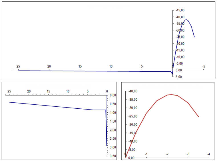
For the evaluation of strains and crack bandwidth, we recommend creating a section for each considered crack band in RFEM. From this section, you can easily find the mean tensile strain and the crack bandwidth. The section must be defined parallel to the displayed strain direction. The crack width perpendicular to the x-axis on the bottom side governs in the analyzed slab. Image 08 shows the created section with the average value for the tensile strains and the integration length.
The existing crack width wk,prov from pure load action (t = 180 days) results in
wk,prov,x = 0.219‰ ⋅ 1.172 m = 0.26 mm <0.3 mm (for the exposition class XC 2).
C) Crack Width Analysis from Load Action and Effects Due to Restraint
The crack width analysis due to load action with restraint from shrinkage results at the end of the working life. When calculating the crack width using the strains from the FEM calculation, it is important to ensure that the strain causing stress is determined in a simple recalculation. The explanation for this can be found in the shrinkage behavior of the plate up to the time t = 180 days. If the plate can contract without constraint, the FEM calculation results in a strain that is equal to the shrinkage strain. The resulting stress is zero in this case. A tensile stress only arises when a "stress-generating strain" εwk,restraint occurs.
|
εwk,zwang |
Strain causing stress |
|
εFEM |
Strain from an FEM calculation |
|
εcs,wk |
Shrinkage strain |
In order to determine the crack bandwidth in RFEM, it is necessary first to determine the strain of the finite element at which the element cracks under the applied restraint.
εcr,FEM,restraint = εcs,wk + εcr = -0.257‰ + 0.1 ‰ = -0.157‰
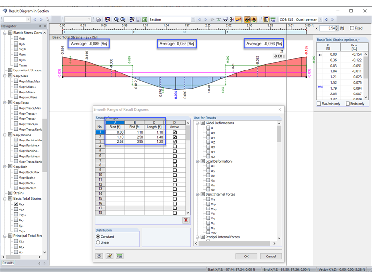
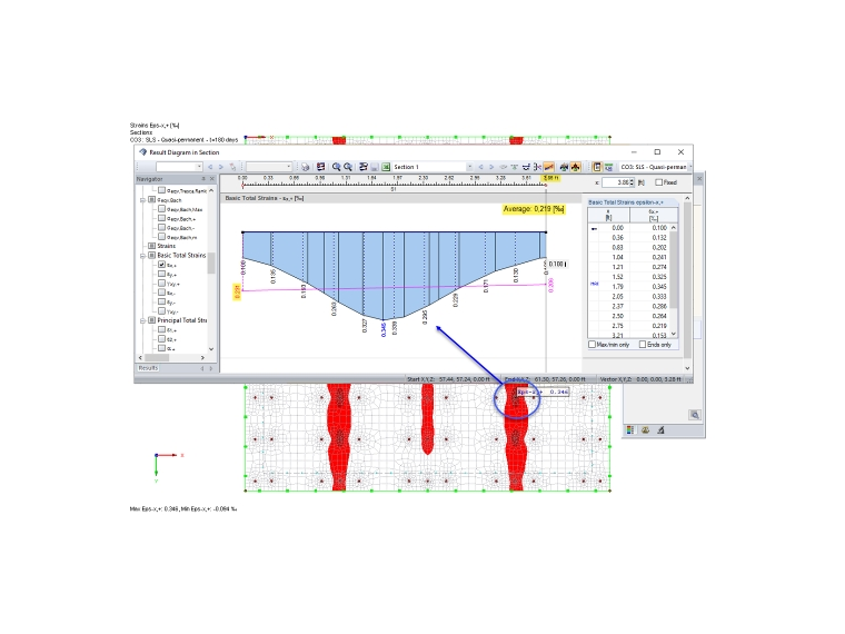
Image 09 shows the governing section for the crack width calculation with load action and effects due to restraint. To integrate the strains across the crack bandwidth, the section must be divided into several areas.
The existing crack width is calculated as follows:
wk,prov,y = (-0.089‰ + 0.257‰) ⋅ 0.335 m + (0.059‰ + 0.257‰) ⋅ 0.450 m + (-0.093‰ + 0.257‰) ⋅ 0.402 m = 0.27 mm < 0.30 mm (for exposition class XC 2)
The crack width could be verified.
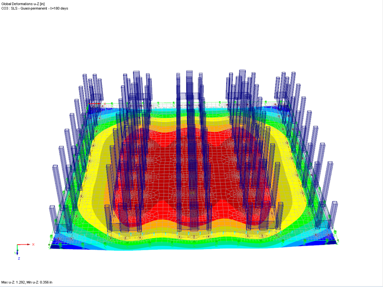
D) Deformation Analysis
The maximum deformations can be taken directly from the RFEM results. The total displacement under the quasi-permanent load is 32.8 mm. The deformation difference of the base plate results from the difference between the minimum and maximum deformations and amounts to 32.8 mm - 9 mm = 23.8 mm (see Image 10).
The allowable limit values and the associated system compatibility for the rack must be agreed with the rack manufacturer.
Finally, we would like to point out the very helpful recommendations for performing nonlinear calculations with the "Isotropic Damage 2D/3D" material model in the technical article about the ultimate limit state design.
