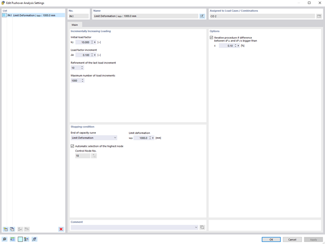
The pushover analysis is managed by a newly introduced analysis type in the load combinations. Here, you have access to the selection of the horizontal load distribution and direction, the selection of a constant load, the selection of the desired response spectrum for the determination of the target displacement, and the pushover analysis settings tailored to the pushover analysis.
In the pushover analysis settings, you can modify the increment of the increasing horizontal load and specify the stopping condition for the analysis. Furthermore, it is possible to easily adjust the precision for the iterative determination of the target displacement.

You have several options available to define masses for a modal analysis. While the masses due to self-weight are considered automatically, you can consider the loads and masses directly in a load case of the modal analysis type. Do you need more options? Select whether to consider full loads as masses, load components in the global Z-direction, or only the load components in the direction of gravity.
The program offers you an additional or alternative option for importing masses: A manual definition of load combinations as of which are the masses considered in the modal analysis. Have you selected a design standard? You can then create a design situation with the Seismic Mass combination type. Thus, the program automatically calculates a mass situation for the modal analysis according to the preferred design standard. In other words: The program creates a load combination on the basis of the preset combination coefficients for the selected standard. This contains the masses used for the modal analysis.

In RFEM, you can use these three powerful eigenvalue solvers:
- Root of Characteristic Polynomial
- Method by Lanczos
- Subspace Iteration
RSTAB, on the other hand, provides you with these two eigenvalue solvers:
- Subspace Iteration
- Shifted inverse power method
The selection of the eigenvalue solver depends primarily on your model size.

- Automatic consideration of masses from self-weight
- Direct import of masses from load cases or load combinations
- Optional definition of additional masses (nodal, linear, or surface masses, as well as inertia masses) directly in the load cases
- Optional neglect of masses (for example, mass of foundations)
- Combination of masses in different load cases and load combinations
- Preset combination coefficients for various standards (EC 8, SIA 261, ASCE 7,...)
- Optional import of initial states (for example, to consider prestress and imperfection)
- Structure Modification
- Consideration of failed supports or members/surfaces/solids
- Definition of several modal analyses (for example, to analyze different masses or stiffness modifications)
- Selection of mass matrix type (diagonal matrix, consistent matrix, unit matrix), including user-defined specification of translational and rotational degrees of freedom
- Methods for determining the number of mode shapes (user-defined, automatic - to reach effective modal mass factors, automatic - to reach the maximum natural frequency - only available in RSTAB)
- Determination of mode shapes and masses in nodes or FE mesh points
- Results of eigenvalue, angular frequency, natural frequency, and period
- Output of modal masses, effective modal masses, modal mass factors, and participation factors
- Masses in mesh points displayed in tables and graphics
- Visualization and animation of mode shapes
- Various scaling options for mode shapes
- Documentation of numerical and graphical results in printout report
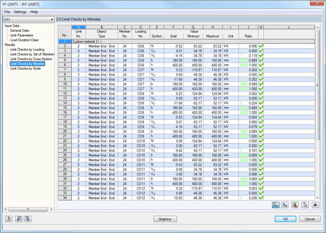
First, the governing design checks of the connection for the respective load case, and load combination, or result combination are displayed. In addition, it is possible to display results separately for sets of members, surfaces, cross-section, members, nodes, and nodal supports.
- You can use a filter to further reduce the displayed results and thus present them in a clearer way.
- Design of hinged, bending resistant, and semi-rigid connections
- Definition of up to 5 steel plates slotted in timber beams
- Up to 8 members connected to one node
- Thickness of steel plate 5 mm – 40 mm
- All sizes of fasteners
- Automatic check of the minimum distance between fasteners
- Optional free definition of fastener distances
- Definition of asymmetrical fastener arrangements (for example, any polygonal chains)
- Graphical visualization of joints in the add-on module and in RFEM/RSTAB
- All required steel and timber designs, including reduction of cross‑section values
- Design of transversal tension reinforcement (for EN 1995‑1‑1 only)
- Export of the member eccentricities to RFEM/RSTAB to be considered in the determination of internal forces
- Dowel length optionally shorter than cross-section width (for wooden plugs)
- DXF Export of Connection Geometry
- Fire resistance design according to EN 1995‑1‑2

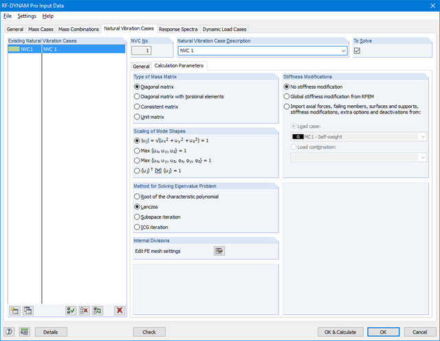
In the modal analysis settings, you have to enter all data that are necessary for the determination of the natural frequencies. These are, for example, mass shapes and eigenvalue solvers.
The Modal Analysis add-on determines the lowest eigenvalues of the structure. Either you adjust the number of eigenvalues or let them determined automatically. Thus, you should reach either effective modal mass factors or maximum natural frequencies. Masses are imported directly from load cases and load combinations. In this case, you have the option to consider the total mass, load components in the global Z-direction, or only the load component in the direction of gravity.
You can manually define additional masses at nodes, lines, members, or surfaces. Furthermore, you can influence the stiffness matrix by importing axial forces or stiffness modifications of a load case or load combination.

Do you want to consider other loads as masses in addition to the static loads? The program allows that for nodal, member, line and surface loads. For this, you need to select the Mass load type when defining the load of interest. Define a mass or mass components in the X, Y, and Z directions for such loads. For nodal masses, you have an additional option to also specify moments of inertia X, Y, and Z in order to model more complex mass points.
- Design of member ends, members, nodal supports, nodes, and surfaces
- Consideration of specified design areas
- Check of cross-section dimensions
- Design according to EN 1995-1-1 (European Timber Standard) with the respective National Annexes + DIN 1052 + DSTV DIN EN 1993-1-8 + ANSI / AWC - NDS 2015 (US Standard)
- Design of various materials, such as steel, concrete, and others
- No necessary linking to specific standards
- Extensible library including timber fasteners (SIHGA, Sherpa, WÜRTH, Simpson StrongTie, KNAPP, PITZL) and steel fasteners (standardized connections in steel building design according to EC 3, M-connect, PFEIFER, TG-Technik)
- Ultimate load capacities of timber beams by the companies STEICO and Metsä Wood available in the library
- Connection to MS Excel
- Optimization of connecting elements (the most utilized element is calculated)

The Dlubal structural analysis software does a lot of work for you. The input parameters, which are relevant for the selected standards, are suggested by the program in accordance with the rules. Furthermore, you can enter response spectra manually.
Load cases of the type Response Spectrum Analysis define the direction in which response spectra act and which eigenvalues of the structure are relevant for the analysis. In the spectral analysis settings, you can define details for the combination rules, damping (if applicable), and zero-period acceleration (ZPA).
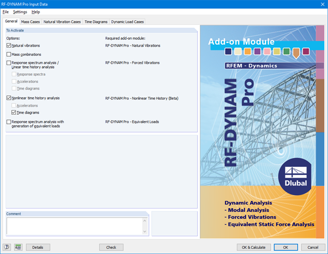
RF-/DYNAM Pro - Nonlinear Time History is integrated in the structure of RF‑/DYNAM Pro - Forced Vibrations and extended by two nonlinear analysis methods (one nonlinear analysis in RSTAB).
Force-time diagrams can be entered as transient, periodic, or as a function of time. Dynamic load cases combine the time diagrams with the static load cases, which provides high flexibility. Furthermore, it is possible to define time steps for the calculation, structural damping, and export options in the dynamic load cases.

As soon as the program has completed the calculation, the eigenvalues, natural frequencies and periods are listed. These result windows are integrated in the main program RFEM/RSTAB. You can find all mode shapes of the structure in tables and also have an option to display them graphically and to animate them.
All result tables and graphics are part of the RFEM/RSTAB printout report. In this way, you can ensure clearly arranged documentation. You can also export the tables to MS Excel.

It is often necessary to neglect masses. This is particularly the case when you want to use the output of the modal analysis for the seismic analysis. For this, 90% of the effective modal mass in each direction is required for the calculation. So you can neglect the mass in all fixed nodal and line supports. The program automatically deactivates the associated masses for you.
You can also manually select the objects whose masses are to be neglected for the modal analysis. We have shown the latter in the image for a better view. A user-defined selection is made the and the objects with their associated mass components are selected to neglect the masses.

You can already see it in the image: Imperfections can also be taken into account when defining a modal analysis load case. The imperfection types that you can use in the modal analysis are notional loads from load case, initial sway via table, static deformation, buckling mode, dynamic mode shape, and group of imperfection cases.

When defining the input data for the modal analysis load case, you can consider a load case whose stiffnesses represent the initial position for the modal analysis. How do you do that? As shown in the image, select the "Consider initial state from" option. Now, open the "Initial State Settings" dialog box and define the type Stiffness as the initial state. In this load case, as of which is the initial state taken into account, you can consider the stiffness of the structural system when the tension members fail. The purpose of all of this: The stiffness from this load case is considered in the modal analysis. Thus, you obtain a clearly flexible system.
- Applicable for members defined as sets of members
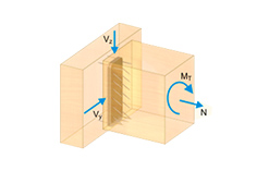
- Separate solver that considers 7 deformation directions (ux, uy, uz, φx, φy, φz, ω) or 8 internal forces (N, Vu, Vv, Mt,pri, Mt,sec, Mu, Mv, Mω)
- Nonlinear design according to second-order analysis
- Input of imperfections
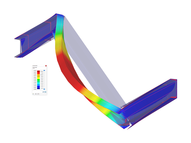
- Calculation of critical load factors and buckling mode shapes as well as the visualization of them (incl. warping)
- Integration into member design in the RF-/STEEL AISC and RF‑/STEEL EC3 add‑on modules
- Available for all thin‑walled steel cross‑sections
- Automatic consideration of masses from self-weight
- Direct import of masses from load cases or load combinations
- Optional definition of additional masses (nodal, linear, surface masses, as well as inertia masses)
- Combination of masses in different mass cases and mass combinations
- Preset combination coefficients according to EC 8
- Optional import of normal force distributions (in order to consider prestress, for example)
- Stiffness modification (for example, deactivated members or stiffnesses can be imported from RF-/CONCRETE)
- Consideration of failed supports or members
- Definition of several natural vibration cases (for example, to analyze different masses or stiffness modifications)
- Results of eigenvalue, angular frequency, natural frequency, and period
- Determination of mode shapes and masses in nodes or FE mesh points
- Results of modal masses, effective modal masses, and modal mass factors
- Visualization and animation of mode shapes
- Various scaling options for mode shapes
- Documentation of numerical and graphical results in the printout report
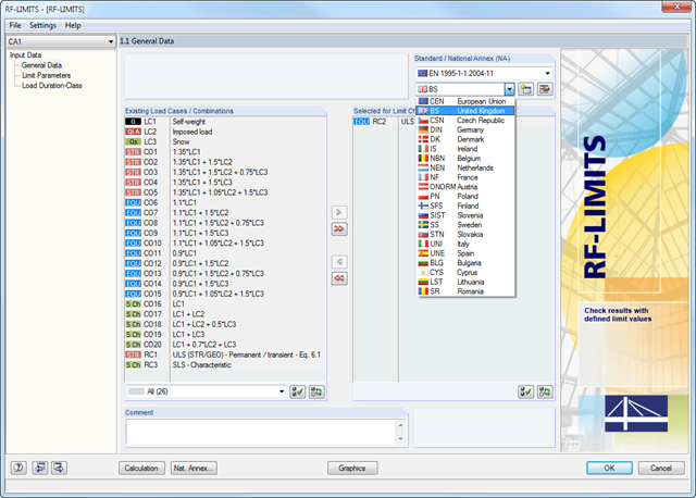
After selecting the loads required for the design and, if necessary, the desired standard for the design, you can define the limit loads in Window 1.2 Limit Parameters. In addition to the manufacturers listed in the limit library, it is possible to add user-defined entries.
After selecting all limit elements for the design, you can optionally define the load duration class (LDC). However, this module window is available only for timber fastener design according to EN 1995-1-1 or DIN 1052.

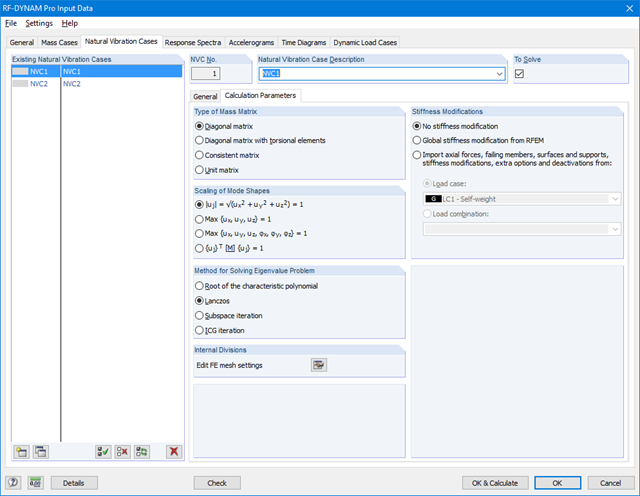
Did you know? You can easily define structural modifications in load cases of the Modal Analysis type. This allows you, for example, to individually adjust the stiffnesses of materials, cross-sections, members, surfaces, hinges, and supports. You can also modify stiffnesses for some design add-ons. Once you select the objects, their stiffness properties are adapted to the object type. In this way, you can define them in separate tabs.
Do you want to analyze the failure of an object (for example, a column) in the modal analysis? This is also possible without any problems. Simply switch to the Structure Modification window and deactivate the relevant objects.
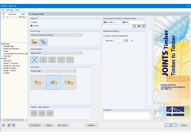
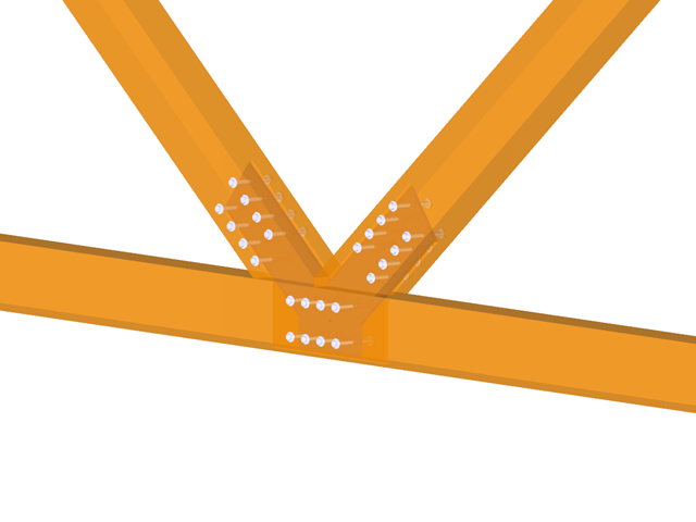
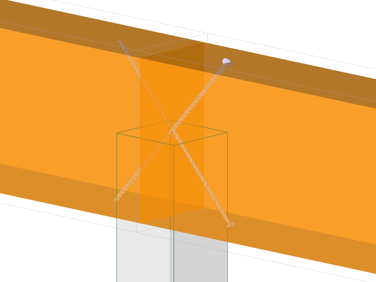
First, select the joint type and the design standard.
The connected members are imported from the RFEM/RSTAB model. The add-on module automatically checks if all geometry conditions are fulfilled.
In addition, the loads are imported automatically from RFEM/RSTAB. In the Geometry window, you can specify the screw parameters (diameter, length, angle, and so on).

The load cases of the type Response Spectrum Analysis contain the generated equivalent loads. First, the modal contributions have to be superimposed with the SRSS or CQC rule. In this case, you can use the signed results based on the dominant mode shape.
Afterwards, the directional components of earthquake actions are combined with the SRSS or the 100% / 30% rule.
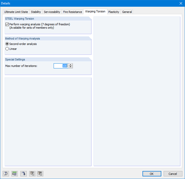
Since RF-/STEEL Warping Torsion is fully integrated in RF-/STEEL AISC and RF‑/STEEL EC3, the data are entered in the same way as for the usual design in these modules. It is only necessary to select the option "Perform warping analysis" in the Details dialog box, tab Warping Torsion (see the figure on the right). You can also define the maximum number of iterations in this dialog box.
The warping torsion analysis is performed for sets of members in RF-/STEEL AISC and RF‑/STEEL EC3. You can define boundary conditions such as nodal supports or member end releases for them.
It is also possible to specify imperfections for the nonlinear calculation.

- Nonlinear member types, such as tension and compression members or cables
- Member nonlinearities, such as failure, tearing, yielding under tension or compression
- Support nonlinearities, such as failure, friction, diagram, and partial activity
- Release nonlinearities, such as friction, partial activity, diagram, and fixed if positive or negative internal forces
Equivalent static loads are generated separately for each relevant eigenvalue and excitation direction. They are exported to static load cases to perform the linear static analysis in RFEM/RSTAB.
The time history analysis is performed with the modal analysis or the linear implicit Newmark analysis. The time history analysis in this add‑on module is restricted to linear systems. Although the modal analysis represents a fast algorithm, it is necessary to use a certain number of eigenvalues to ensure the required accuracy of results.
The implicit Newmark analysis is a very precise method, independent of the number of eigenvalues used, but requires sufficient small time steps for calculation. For the response spectra analysis, equivalent static loads are calculated internally. A linear static analysis is performed subsequently.
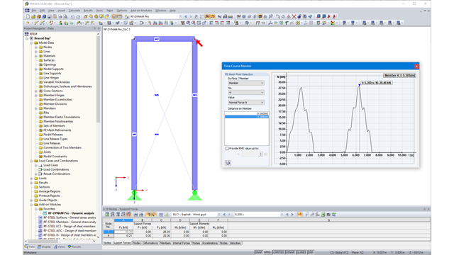
Due to the integration of RF‑/DYNAM Pro in RFEM or RSTAB, you can incorporate numeric and graphic results from RF‑/DYNAM Pro - Nonlinear Time History to the global printout report. Also, all RFEM and RSTAB options are available for a graphical visualization. The results of the time history analysis are displayed in a time history diagram.
The results are displayed as a function of time and the numerical values can be exported to MS Excel. Result combinations can be exported, either as a result of a single time step or the most unfavorable results of all time steps are filtered out.
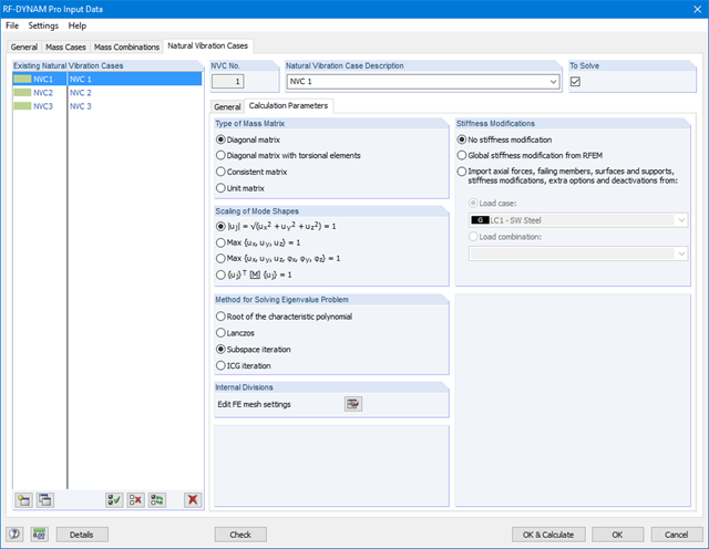
The RF-DYNAM Pro - Natural Vibrations module of RFEM provides four powerful eigenvalue solvers:*Root of characteristic polynomial
- Method by Lanczos
- Subspace Iteration
- ICG iteration method (Incomplete Conjugate Gradient)
The DYNAM Pro - Natural Vibrations module for RSTAB provides two eigenvalue solvers:
- Subspace Iteration
- Shifted inverse power method
The selection of the eigenvalue solver depends primarily on the size of the model.
.png?mw=640&hash=c1087880acc023575381bb136280b0c348568350)
- Design of hinged connections
- Biaxial inclination of the connected member (for example, a jack rafter joint)
- Connection of any number of members on one node for the type "Main member only"
- Screw diameter 6 mm – 12 mm
- Automatic check of the minimum distance between screws
- Optional free definition of screw distances
- Transfer of eccentricity from RFEM/RSTAB
- Crosswise or parallel screw alignment
- Definition of up to 16 screws in a row
- Graphical visualization of joints in the add-on module and in RFEM/RSTAB
- Performing all required designs
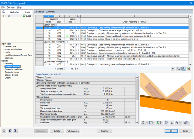
At first, the governing joint designs are arranged in groups and displayed with the basic geometry of the joint in the first result window. In the other result windows, you can see all fundamental design details.
Dimensions, material properties, and welds important for the connection construction are displayed immediately and can be printed directly. Similarly, export to DXF-file is enabled. It is possible to visualize the connections in RF‑/JOINTS Timber - Steel to Timber or in the RFEM/RSTAB model.
All graphics can be included in the RFEM/RSTAB printout report or printed directly. Due to the scaled output, an optimal visual check is possible as early as in the design phase.
.png?mw=640&hash=8cfd0c4bd093c03de543d147ffbf6f5c9250634a)
- User-defined time diagrams as a function of time, in tabular form, or as harmonic loads
- Combination of the time diagrams with RFEM/RSTAB load cases or combinations (enables definition of nodal, member, and surface loads, as well as free and generated loads varying over time)
- Combination of several independent excitation functions
- Nonlinear time history analysis with the implicit Newmark analysis (RFEM only) or the explicit analysis
- Structural damping using Rayleigh damping coefficients or Lehr's damping
- Direct import of initial deformations from a load case or combination (RFEM only)
- Stiffness modifications as initial conditions; for example, axial force effect, deactivated members (RSTAB only)
- Graphical display of results in a time history diagram
- Export of results in user-defined time steps or as an envelope