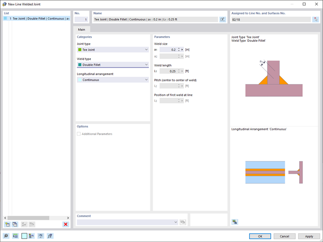
In RFEM 6, it is possible to define line welds between surfaces and to calculate the weld stresses using the Stress-Strain Analysis add-on.
The following joint types are available:
- Butt Joint
- Corner joint
- Lap Joint
- T-joint
Depending on the selected joint type, you can select the following weld types:
- Single Square
- Double Square
- Double Bevel
- Single V
- Double V
- Single U
- Double U
- Single J
- Double J

Compared to the RF‑/STEEL add-on module (RFEM 5 / RSTAB 8), the following new features have been added to the Stress-Strain Analysis add-on for RFEM 6 / RSTAB 9:
- Treatment of members, surfaces, solids, welds (line welded joints between two and three surfaces with subsequent stress design)
- Output of stresses, stress ratios, stress ranges, and strains
- Limit stress depending on the assigned material or a user-defined input
- Individual specification of the results to be calculated through freely assignable setting types
- Non-modal result details with prepared formula display and additional result display on the cross-section level of members
- Output of the design check formulas used

After you have completed the design, the program takes care of clearly arranged results. Thus, the program shows you the resulting maximum stresses and stress ratios sorted by section, member/surface, solid, member set, x-location, and so on. In addition to the tabular result values, the add-on shows you the corresponding cross-section graphic with stress points, stress diagram, and values as well. You can relate the design ratio to any kind of stress type. The current location is highlighted in the RFEM/RSTAB model.
In addition to the tabular evaluation, the program offers you even more. You can also graphically check the stresses and design ratios on the RFEM/RSTAB model. It is possible for you to adjust the colors and values individually.
The display of result diagrams of a member or set of members enables you a targeted evaluation. For each design location, you can open the respective dialog box to check the design-relevant section properties and stress components of any stress point. Finally, you have the option of printing the corresponding graphic, including all design details.

Are you ready for the evaluation? Use the calculation diagrams, which show the distribution of a specific result during the calculation.
You can freely define the layout of the vertical and horizontal axes of the calculation diagram. This allows you, for example, to consider the settlement distribution of a certain node, depending on the load.

Do you want to model and analyze the behavior of a soil solid? To ensure this, special suitable material models have been implemented in RFEM.
You can use the modified Mohr-Coulomb model with a linear-elastic ideal-plastic model or a nonlinear elastic model with an oedometric stress-strain relation. The limit criterion, which describes the transition from the elastic area to that of the plastic flow, is defined according to Mohr-Coulomb.

Compared to the RF‑SOILIN add-on module (RFEM‑5), the following new features have been added to the Geotechnical Analysis add-on for RFEM 6:
- Creation of the layered soil as a 3D model from the entirety of the defined soil samples
- Recognized material law according to Mohr-Coulomb for soil simulation
- Graphical and tabular output of stresses and strains at any depth of the soil
- Optimal consideration of the soil-structure interaction on the basis of an overall model

You can select several methods that are available for the eigenvalue analysis:
- Direct Methods
- The direct methods (Lanczos [RFEM], roots of characteristic polynomial [RFEM], subspace iteration method [RFEM/RSTAB], and shifted inverse iteration [RSTAB]) are suitable for small to medium-sized models. You should only use these fast solver methods if your computer has a larger amount of memory (RAM).
- ICG Iteration Method (Incomplete Conjugate Gradient [RFEM])
- In contrast, this method only requires a small amount of memory. Eigenvalues are determined one after the other. It can be used to calculate large structural systems with few eigenvalues.
Use the Structure Stability add-on to perform a nonlinear stability analysis using the incremental method. This analysis delivers close-to-reality results also for nonlinear structures. The critical load factor is determined by gradually increasing the loads of the underlying load case until the instability is reached. The load increment takes into account nonlinearities such as failing members, supports and foundations, and material nonlinearities. After increasing the load, you can optionally perform a linear stability analysis on the last stable state in order to determine the stability mode.

The soil solids that you want to analyze are summarized in soil massifs.
Use the soil samples as a basis for a definition of the respective soil massif. This way, the program allows for user-friendly generation of the massif, including the automatic determination of the layer interfaces from the sample data, as well as the groundwater level and the boundary surface supports.
Soil massifs provide you with the option to specify a target FE mesh size independently of the global setting for the rest of the structure. You can thus consider the various requirements of the building and soil in the entire model.

Your data are always documented in a multilingual printout report. You can adjust the content at any time and save it as a template. You can also add graphics, texts, MathML formulas, and PDF documents to your report with just a few clicks.

Compared to the RF‑/STABILITY (RFEM 5) and RSBUCK (RSTAB 8) add-on modules, the following new features have been added to the Structure Stability add-on for RFEM 6 / RSTAB 9:
- Activation as a property of a load case or a load combination
- Automated activation of the stability calculation via combination wizards for several load situations in one step
- Incremental load increase with user-defined termination criteria
- Modification of the mode shape normalization without recalculation
- Result tables with filter option
.png?mw=640&hash=55038d2a1591f62179796666cb9b2fede0274e19)
A graphical and tabular output of the results for deformations, stresses, and strains helps you when determining the soil solids. To achieve this, use the special filter criteria for targeted selection of results.
The program doesn't leave you alone with the results. If you want to graphically evaluate the results in the soil solids, you can use the guide objects. For example, you can define clipping planes. This allows you to view the corresponding results in any plane of the soil solid.
And not just that. The utilization of result sections and clipping boxes facilitates the precise graphical analysis of the soil solid.
You already know that it is possible to model and analyze a soil and a structure in the entire model. As a result, you have explicitly taken into account the soil-structure interaction. By modifying a component, you achieve the immediate correct consideration in the analysis as well as in the results for the entire system of the soil and structure.

As the first results, the program presents you with the critical load factors. You can then perform an evaluation of stability risks. For member models, the resulting effective lengths and critical loads of the members are displayed to you in tables.
Use the next result window to check the normalized eigenvalues sorted by node, member, and surface. The eigenvalue graphic allows you to evaluate the buckling behavior. This makes it easier for you to take countermeasures.
- Determination of principal and basic stresses, membrane and shear stresses, as well as equivalent stresses and equivalent membrane stresses
- Stress analysis for structural surfaces including simple or complex shapes
- Equivalent stresses calculated according to different approaches:
- Shape modification hypothesis (von Mises)
- Shear stress hypothesis (Tresca)
- Normal stress hypothesis (Rankine)
- Principal strain hypothesis (Bach)
- Optional optimization of surface thicknesses and data transfer to RFEM
- Output of strains
- Detailed results of individual stress components and ratios in tables and graphics
- Filter function for solids, surfaces, lines, and nodes in tables
- Transversal shear stresses according to Mindlin, Kirchhoff, or user-defined specifications
- Stress evaluation for welds at connection lines between surfaces (see the Product Feature)

You can be sure that costs are an important factor in the structural planning of any project. It is also essential to adhere to the provisions on emissions estimation. The two-part add-on Optimization & Costs/CO2 Emission Estimation makes it easier for you to find your way through the jungle of standards and options. It uses the artificial intelligence technology (AI) of the particle swarm optimization (PSO) to find the right parameters for parameterized models and blocks that guarantee the compliance with the usual optimization criteria. This add-on also estimates the model costs or CO2 emissions by specifying unit costs or emissions per material definition for the structural model. With this add-on, you are on the safe side.

Did you know? You can enter the soil layers that you have obtained from the subsoil expertises done in the locations into the program in the form of soil samples. Assign the explored soil materials, including their material properties, to the layers.
For the definition of the samples, you can enter the data in tables as well as in the respective editing dialog box. Furthermore, you can also specify the groundwater level in the soil samples.
Entering soil layers for soil samples is performed in a clearly arranged dialog box. A corresponding graphical representation supports clarity and makes checking the input user-friendly.
An extensible database facilitates the selection of soil material properties. The Mohr-Coulomb model as well as a nonlinear model with stress and strain dependent stiffness are available for a realistic modeling of the soil material behavior.
You can define any number of soil samples and layers. The soil is generated from all entered samples using 3D solids. Assignment to the structure is carried out using coordinates.
The soil body is calculated according to the nonlinear iterative method. The calculated stresses and settlements are displayed graphically and in tables.
If there is a load case or load combination in the program, the stability calculation is activated. You can define another load case in order to consider initial prestress, for example.
For this, you need to specify whether to perform a linear or nonlinear analysis. Depending on the case of application, you can select a direct calculation method, such as the Lanczos method or the ICG iteration method. Members not integrated in surfaces are usually displayed as member elements with two FE nodes. With such elements, the program cannot determine the local buckling of single members. That's why you have the option to divide members automatically.

- Calculation of models consisting of member, shell, and solid elements
- Nonlinear stability analysis
- Optional consideration of axial forces from initial prestress
- Four equation solvers for an efficient calculation of various structural models
- Optional consideration of stiffness modifications in RFEM/RSTAB
- Determination of a stability mode greater than the user-defined load increment factor (Shift method)
- Optional determination of the mode shapes of unstable models (to identify the cause of instability)
- Visualization of the stability mode
- Basis for determining imperfection

- General stress analysis
- Automatic import of internal forces from RFEM/RSTAB
- Graphical and numerical output of stresses, strains, clearance, and design ratios fully integrated in RFEM/RSTAB
- User-defined specification of the limit stress
- Summary of similar structural components for the design
- Wide range of customization options for graphical output
- Clearly arranged result tables for a quick overview after the design
- Simple traceability of the results due to the complete documentation of the calculation method including all formulas
- High productivity due to the minimal amount of input data required
- Flexibility due to detailed setting options for basis and extent of calculations
- Gray zone display for unimportant value ranges (see Product Feature)