
When generating shear walls and deep beams, you can assign not only surfaces and cells, but also members.

You can neglect openings with a certain area in the building model calculation. This function can be activated in the global settings of the building stories. A warning message appears saying that the openings have been neglected.

Both optimization methods have one thing in common. At the end of the process, they provide you with a list of model mutations from the stored data. Here you can find the details of the controlling optimization result and the associated value assignment of the optimization parameters. This list is organized in descending order. You can find the assumed best solution shown in the first line. For this, the optimization result with its determined value assignment is closest to the optimization criterion. All add-on results have a utilization < 1. Furthermore, once the analysis is completed, the program will adjust the value assignment to that of the optimal solution for the optimization parameters in the global parameter list.
In the material dialog boxes, you can find the additional tabs "Cost Estimation" and "Estimation of CO2 Emissions". They show you the individual estimated sums of the assigned members, surfaces, and solids per unit weight, volume, and area. Furthermore, these tabs show the total cost and emission of all assigned materials. This gives you a good overview of your project.
The building story generator in the Building Model add-on allows you to automatically create building stories, depending on the topology of the model.

For a response spectrum analysis of building models, you can display the sensitivity coefficients for the horizontal directions by story.
These key figures allow you to interpret the sensitivity to stability effects.

Did you know? The structural optimization in the programs RFEM and RSTAB is a completion of the parametric input. It is a parallel process beside the actual model calculation with all its regular calculation and design definitions. The add-on assumes that your model or block is built with a parametric context and is controlled in its entirety by global control parameters of the "optimization" type. Therefore, these control parameters have a lower and upper limit and a step size to delimit the optimization range. If you want to find optimal values for the control parameters, you have to specify an optimization criterion (for example, minimum weight) with the selection of an optimization method (for example, particle swarm optimization).
You can already find the cost and CO2 emission estimation in the material definitions. You can activate both options individually in each material definition. The estimation is based on a unit for unit cost or unit emission for members, surfaces, and solids. In this case, you can select whether to specify the units by weight, volume, or area.

You can display the results as usual via the Results navigator. Furthermore, the dialog box of the add-on shows you the information about the individual floors. Thus, you always have a good overview.

- Artificial intelligence technology (AI): Particle swarm optimization (PSO)
- Structure optimization according to the minimum weight or deformation
- Use of any number of optimization parameters
- Specification of variable ranges
- Optimization of cross-sections and materials
- Parameter definition types
- Optimization | Ascending or Optimization | Descending
- Application of parametric models and blocks
- Code-based JavaScript parametrization of blocks
- Optimization taking into account the design results
- Tabular display of the best model mutations
- Real-time display of the model mutations in the optimization process
- Model cost estimation by specifying unit prices
- Determination of the global warming potential GWP when realizing the model by estimating the CO2 equivalent
- Specification of weight-, volume-, and area-based units (price and CO2e)
You have two options for a building model. You can create it when you start modeling the structure, or activate it afterwards. In the building model, you can then directly define the stories and manipulate them.
When manipulating the stories, you can choose whether to modify or retain the included structural elements using various options.
RFEM does some of the work for you. For example, it automatically generates result sections, so you don't need to perform a lot of calculations.
Shear walls and deep beams of a building model are available as independent objects in the design add-ons. This allows for faster filtering of the objects in results, as well as better documentation in the printout report.

There are two methods that you can use for the optimization process, with which you can find optimal parameter values according to a weight or deformation criterion.
The most efficient method with the littlest calculation time is the near-natural particle swarm optimization (PSO). Have you heard or read about it? This artificial intelligence (AI) technology has a strong analogy to the behavior of flocks of animals, looking for a resting place. In such swarms, you can find many individuals (cf. optimization solution - for example, weight) who like to stay in a group and follow the group movement. Let's assume that each individual swarm member has a need to rest at an optimal resting place (cf. best solution - for example, lowest weight). This need increases as the resting place is approached. Thus, the swarm behavior is also influenced by the properties of the space (cf. result diagram).
Why the excursion into biology? Quite simply – the PSO process in RFEM or RSTAB proceeds in a similar way. The calculation run starts with an optimization result from a random assignment of the parameters to be optimized. It repeatedly determines new optimization results with varied parameter values, which are based on the experience of the previously performed model mutations. The process continues until the specified number of possible model mutations is reached.
As an alternative to this method, the program also offers you a batch processing method. This method attempts to check all possible model mutations by randomly specifying the values for the optimization parameters until a predetermined number of possible model mutations is reached.
After calculating a model mutation, both variants also check the respective activated design results of the add-ons. Furthermore, they save the variant with the corresponding optimization result and value assignment of the optimization parameters if the utilization is < 1.
You can determine the estimated total costs and emission from the respective sums of the individual materials. The sums of the materials are composed of the weight-based, volume-based, and area-based partial sums of the member, surface, and solid elements.

The modal relevance factor (MRF) can help you to assess to which extent specific elements participate in a specific mode shape. The calculation is based on the relative elastic deformation energy of each individual member.
The MRF can be used to distinguish between local and global mode shapes. If multiple individual members show significant MRF (for example, > 20%), the instability of the entire structure or a substructure is very likely. On the other hand, if the sum of all MRFs for an eigenmode is around 100%, a local stability phenomenon (for example, buckling of a single bar) can be expected.
Furthermore, the MRF can be used to determine critical loads and equivalent buckling lengths of certain members (for example, for stability design). Mode shapes for which a specific member has small MRF values (for example, < 20%) can be neglected in this context.
The MRF is displayed by mode shape in the result table under Stability Analysis → Results by Members → Effective Lengths and Critical Loads.

- Consideration and display of story masses
- Listing of structural elements and their information
- Automated creation of result sections on shear walls
- Output of section resultants in global direction for determining shear forces
- Optional definition of rigid diaphragm by story (story modeling)
- Stiffness type Floor Slab - Rigid Diaphragm
- Defining floor sets,
- for example, calculation of slabs as a 2D position within the 3D model
- Shear walls: Automatic definition of result members with any cross-section
- Design of rectangular cross-sections using the Concrete Design add-on
- Definition of deep beams
- Design with the Concrete Design add-on
- Tabular output of story actions, interstory drift, and center points of mass and stiffness, as well as the forces in shear walls
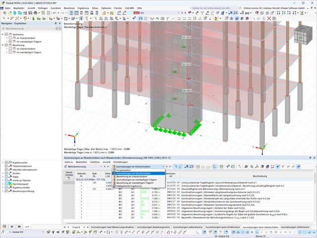
- Separate result display of the floor and stiffening design
- Optional neglecting of openings of a certain size

- Calculation of models consisting of member, shell, and solid elements
- Nonlinear stability analysis
- Optional consideration of axial forces from initial prestress
- Four equation solvers for an efficient calculation of various structural models
- Optional consideration of stiffness modifications in RFEM/RSTAB
- Determination of a stability mode greater than the user-defined load increment factor (Shift method)
- Optional determination of the mode shapes of unstable models (to identify the cause of instability)
- Visualization of the stability mode
- Basis for determining imperfection

If there is a load case or load combination in the program, the stability calculation is activated. You can define another load case in order to consider initial prestress, for example.
For this, you need to specify whether to perform a linear or nonlinear analysis. Depending on the case of application, you can select a direct calculation method, such as the Lanczos method or the ICG iteration method. Members not integrated in surfaces are usually displayed as member elements with two FE nodes. With such elements, the program cannot determine the local buckling of single members. That's why you have the option to divide members automatically.
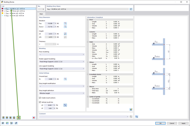
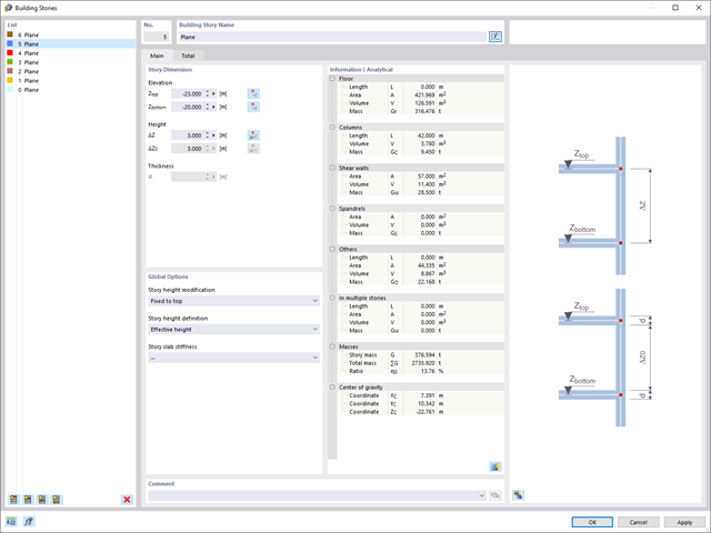
Are you afraid that your project will end in the digital tower of Babel? The Building Model add-on for RFEM supports you in your work on a construction project with several stories. It allows you to define a building by means of stories at specified elevations. You can adjust the stories in many ways afterwards and also select the story slab stiffness. Information about the stories and the entire model (center of gravity, center of rigidity) is displayed for you in tables and graphics.

Several modeling tools are available for elements in building models:
- Vertical line
- Column
- Wall
- Beam
- Rectangular floor
- Polygonal floor
- Rectangular floor opening
- Polygonal floor opening
This feature allows you to define the element on the ground plane (for example, with a background layer) with the associated multiple element creation in space.

You can be sure that costs are an important factor in the structural planning of any project. It is also essential to adhere to the provisions on emissions estimation. The two-part add-on Optimization & Costs/CO2 Emission Estimation makes it easier for you to find your way through the jungle of standards and options. It uses the artificial intelligence technology (AI) of the particle swarm optimization (PSO) to find the right parameters for parameterized models and blocks that guarantee the compliance with the usual optimization criteria. This add-on also estimates the model costs or CO2 emissions by specifying unit costs or emissions per material definition for the structural model. With this add-on, you are on the safe side.

As the first results, the program presents you with the critical load factors. You can then perform an evaluation of stability risks. For member models, the resulting effective lengths and critical loads of the members are displayed to you in tables.
Use the next result window to check the normalized eigenvalues sorted by node, member, and surface. The eigenvalue graphic allows you to evaluate the buckling behavior. This makes it easier for you to take countermeasures.

Using the "Load Transfer Only" story type, you can consider slabs without stiffness effect in and out of the plane in the Building Model add-on. This element type collects the loads on the slab and transfers them to the supporting elements of a 3D model. Thus, you can simulate secondary components, such as grillage and similar load distribution elements, without any further effect in the 3D model.
Compared to the RF‑/STABILITY (RFEM 5) and RSBUCK (RSTAB 8) add-on modules, the following new features have been added to the Structure Stability add-on for RFEM 6 / RSTAB 9:
- Activation as a property of a load case or a load combination
- Automated activation of the stability calculation via combination wizards for several load situations in one step
- Incremental load increase with user-defined termination criteria
- Modification of the mode shape normalization without recalculation
- Result tables with filter option

You can select several methods that are available for the eigenvalue analysis:
- Direct Methods
- The direct methods (Lanczos [RFEM], roots of characteristic polynomial [RFEM], subspace iteration method [RFEM/RSTAB], and shifted inverse iteration [RSTAB]) are suitable for small to medium-sized models. You should only use these fast solver methods if your computer has a larger amount of memory (RAM).
- ICG Iteration Method (Incomplete Conjugate Gradient [RFEM])
- In contrast, this method only requires a small amount of memory. Eigenvalues are determined one after the other. It can be used to calculate large structural systems with few eigenvalues.
Use the Structure Stability add-on to perform a nonlinear stability analysis using the incremental method. This analysis delivers close-to-reality results also for nonlinear structures. The critical load factor is determined by gradually increasing the loads of the underlying load case until the instability is reached. The load increment takes into account nonlinearities such as failing members, supports and foundations, and material nonlinearities. After increasing the load, you can optionally perform a linear stability analysis on the last stable state in order to determine the stability mode.

Have you activated the Building Model add-on? Very good! This allows you to display the center of rigidity in tabular and graphical form. Use it for your dynamic analysis, for example.

The building model is calculated in two phases:
- Global 3D calculation of the global model, where the slabs are modeled as a rigid plane (diaphragm) or as a bending plate
- Local 2D calculation of the individual floors
After the calculation, the results of the columns and walls from the 3D calculation and the results of the slabs from the 2D calculation are combined in a single model. This means that there is no need to switch between the 3D model and the individual 2D models of the slabs. The user only works with one model, saves valuable time, and avoids possible errors in the manual data exchange between the 3D model and the individual 2D ceiling models.
The vertical surfaces in the model can be divided into shear walls and opening lintels. The program automatically generates internal result members from these wall objects, so they can be designed as members according to any standard in the Concrete Design add-on.