
- Realistic representation of interaction between a building and soil
- Realistic representation of the influences of the foundation components on each other
- Extensible library of soil properties
- Consideration of several soil samples (probes) at different locations, even outside the building
- Determination of settlements and stress diagrams as well as their graphical and tabular display

Entering soil layers for soil samples is performed in a clearly arranged dialog box. A corresponding graphical representation supports clarity and makes checking the input user-friendly.
An extensible database facilitates the selection of soil material properties. The Mohr-Coulomb model as well as a nonlinear model with stress and strain dependent stiffness are available for a realistic modeling of the soil material behavior.
You can define any number of soil samples and layers. The soil is generated from all entered samples using 3D solids. Assignment to the structure is carried out using coordinates.
The soil body is calculated according to the nonlinear iterative method. The calculated stresses and settlements are displayed graphically and in tables.

- Artificial intelligence technology (AI): Particle swarm optimization (PSO)
- Structure optimization according to the minimum weight or deformation
- Use of any number of optimization parameters
- Specification of variable ranges
- Optimization of cross-sections and materials
- Parameter definition types
- Optimization | Ascending or Optimization | Descending
- Application of parametric models and blocks
- Code-based JavaScript parametrization of blocks
- Optimization taking into account the design results
- Tabular display of the best model mutations
- Real-time display of the model mutations in the optimization process
- Model cost estimation by specifying unit prices
- Determination of the global warming potential GWP when realizing the model by estimating the CO2 equivalent
- Specification of weight-, volume-, and area-based units (price and CO2e)

Did you know? The structural optimization in the programs RFEM and RSTAB is a completion of the parametric input. It is a parallel process beside the actual model calculation with all its regular calculation and design definitions. The add-on assumes that your model or block is built with a parametric context and is controlled in its entirety by global control parameters of the "optimization" type. Therefore, these control parameters have a lower and upper limit and a step size to delimit the optimization range. If you want to find optimal values for the control parameters, you have to specify an optimization criterion (for example, minimum weight) with the selection of an optimization method (for example, particle swarm optimization).
You can already find the cost and CO2 emission estimation in the material definitions. You can activate both options individually in each material definition. The estimation is based on a unit for unit cost or unit emission for members, surfaces, and solids. In this case, you can select whether to specify the units by weight, volume, or area.

There are two methods that you can use for the optimization process, with which you can find optimal parameter values according to a weight or deformation criterion.
The most efficient method with the littlest calculation time is the near-natural particle swarm optimization (PSO). Have you heard or read about it? This artificial intelligence (AI) technology has a strong analogy to the behavior of flocks of animals, looking for a resting place. In such swarms, you can find many individuals (cf. optimization solution - for example, weight) who like to stay in a group and follow the group movement. Let's assume that each individual swarm member has a need to rest at an optimal resting place (cf. best solution - for example, lowest weight). This need increases as the resting place is approached. Thus, the swarm behavior is also influenced by the properties of the space (cf. result diagram).
Why the excursion into biology? Quite simply – the PSO process in RFEM or RSTAB proceeds in a similar way. The calculation run starts with an optimization result from a random assignment of the parameters to be optimized. It repeatedly determines new optimization results with varied parameter values, which are based on the experience of the previously performed model mutations. The process continues until the specified number of possible model mutations is reached.
As an alternative to this method, the program also offers you a batch processing method. This method attempts to check all possible model mutations by randomly specifying the values for the optimization parameters until a predetermined number of possible model mutations is reached.
After calculating a model mutation, both variants also check the respective activated design results of the add-ons. Furthermore, they save the variant with the corresponding optimization result and value assignment of the optimization parameters if the utilization is < 1.
You can determine the estimated total costs and emission from the respective sums of the individual materials. The sums of the materials are composed of the weight-based, volume-based, and area-based partial sums of the member, surface, and solid elements.

Both optimization methods have one thing in common. At the end of the process, they provide you with a list of model mutations from the stored data. Here you can find the details of the controlling optimization result and the associated value assignment of the optimization parameters. This list is organized in descending order. You can find the assumed best solution shown in the first line. For this, the optimization result with its determined value assignment is closest to the optimization criterion. All add-on results have a utilization < 1. Furthermore, once the analysis is completed, the program will adjust the value assignment to that of the optimal solution for the optimization parameters in the global parameter list.
In the material dialog boxes, you can find the additional tabs "Cost Estimation" and "Estimation of CO2 Emissions". They show you the individual estimated sums of the assigned members, surfaces, and solids per unit weight, volume, and area. Furthermore, these tabs show the total cost and emission of all assigned materials. This gives you a good overview of your project.
Compared to the RF‑SOILIN add-on module (RFEM‑5), the following new features have been added to the Geotechnical Analysis add-on for RFEM 6:
- Creation of the layered soil as a 3D model from the entirety of the defined soil samples
- Recognized material law according to Mohr-Coulomb for soil simulation
- Graphical and tabular output of stresses and strains at any depth of the soil
- Optimal consideration of the soil-structure interaction on the basis of an overall model

You can be sure that costs are an important factor in the structural planning of any project. It is also essential to adhere to the provisions on emissions estimation. The two-part add-on Optimization & Costs/CO2 Emission Estimation makes it easier for you to find your way through the jungle of standards and options. It uses the artificial intelligence technology (AI) of the particle swarm optimization (PSO) to find the right parameters for parameterized models and blocks that guarantee the compliance with the usual optimization criteria. This add-on also estimates the model costs or CO2 emissions by specifying unit costs or emissions per material definition for the structural model. With this add-on, you are on the safe side.

Reinforced concrete usually answers the question "How much can you carry?" simply with "Yes". Nevertheless, you need a three-dimensional moment-moment-axial force interaction diagram for the graphical output of the ultimate limit state of reinforced concrete cross-sections. The Dlubal structural analysis software offers you just that.
With the additional display of the load action, you can easily recognize or visualize whether the limit resistance of a reinforced concrete cross-section is exceeded. Since you can control the diagram properties, you can customize the appearance of the My-Mz-N diagram to suit your needs.

Did you know that you can also display the moment-axial force interaction diagrams (M‑N diagrams) graphically? This allows you to display the cross-section resistance in the case of an interaction of a bending moment and an axial force. In addition to the interaction diagrams related to the cross-section axes (My‑N diagram and Mz‑N diagram), you can also generate an individual moment vector to create an Mres‑N interaction diagram. You can display the section plane of the M‑N diagrams in the 3D interaction diagram. The program displays the corresponding value pairs of the ultimate limit state in a table. The table is dynamically linked to the diagram so that the selected limit point is also displayed in the diagram.

Do you want to determine the biaxial bending resistance of a reinforced concrete cross-section? For this, you have to activate a moment-moment interaction diagram (My-Mz diagram) first. This My-Mz diagram represents a horizontal section through the three-dimensional diagram for the specified axial force N. Due to the coupling to the 3D interaction diagram, you can also visualize the section plane there.
.png?mw=640&hash=5a991f211d984ac624978f514e70c53da263e5d9)
Depending on the axial force N, you can generate a moment curvature line for any moment vector. The program also shows you the value pairs of the displayed diagram in a table. Furthermore, you can activate the secant stiffness and tangent stiffness of the reinforced concrete cross-section, belonging to the moment curvature diagram, as an additional diagram.
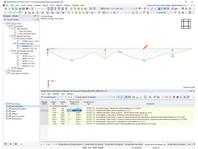
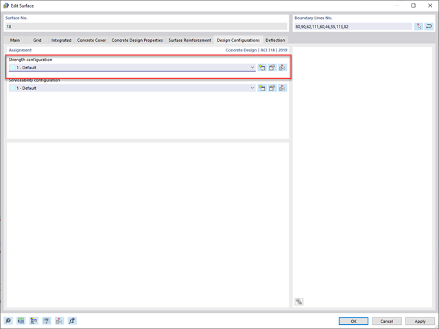
The structural analysis program provides you with a clear overview of all performed design checks for the design standard. You have to determine a design criterion for each design check. In addition to the ultimate limit state and the serviceability limit state design, the program checks the design rules of the standard. For each design check, there are the design details including the initial values, intermediate results, and final results, arranged in a structured way. An information window in the design details shows you the calculation process with the applied formulas, standard sources, and results in great detail.
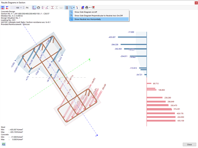
You can display the existing stresses and strains of a concrete cross-section and the reinforcement as a 3D stress image or 2D graphic. Depending on which results do you select in the result tree of the design details, the stresses or strains are displayed to you in the defined longitudinal reinforcement under the load actions or the limit internal forces.
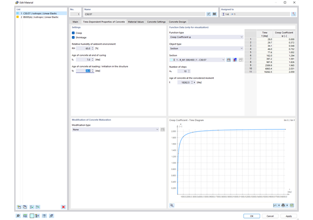
Time-dependent concrete properties, such as creep and shrinkage, are very important for your calculation. You can define them directly for the material in the structural analysis program. In the input dialog box, the time course of the creep or shrinkage function is displayed to you graphically. You can easily select the modification of the applied concrete age, for example, due to a temperature treatment.
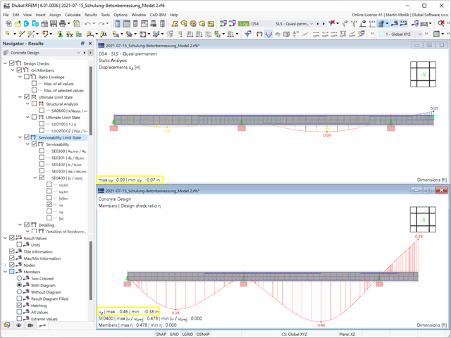
You determine the deformation for members and surfaces, taking into account the cracked (state II) or non-cracked (state I) reinforced concrete cross-section. When determining the stiffness, you can consider "tension stiffening" between the cracks according to the design standard used.
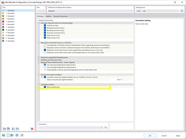
During the cross-section design, you can directly control whether the concrete surface is applied behind the reinforcing bars or is subtracted from the concrete cross-section. You can use the design of the net concrete cross-section especially in the case you deal with a highly reinforced cross-section.
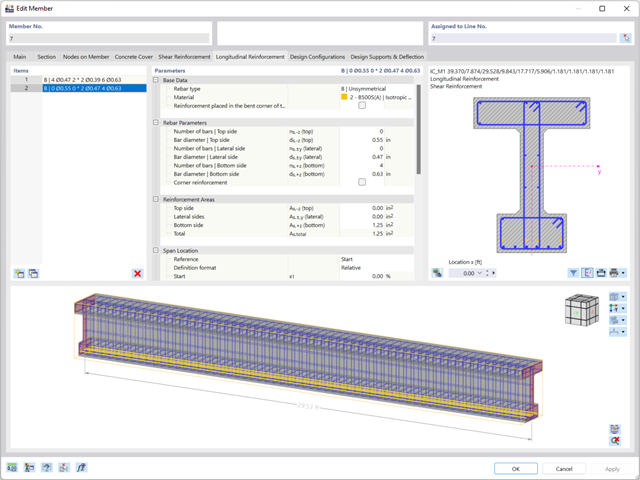
You can specify the shear and longitudinal reinforcement individually for each member. In this case, there are various templates available for entering the reinforcement.
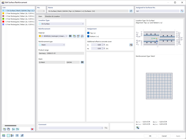
Enter the surface reinforcement directly on the RFEM level. In this case, you can select the defined area reinforcements individually. The usual editing functions Copy, Mirror, or Rotate are at your disposal when entering the surface reinforcement.
.png?mw=640&hash=3c928fddb4215c3df06e0b731d5c3f2e475cd9db)
Within a member, you can define the integration width and effective slab width of T-beams (ribs) with different widths. The member is divided into segments. You can either grade or specify the transition between the different flange widths as linearly variable. Furthermore, the program allows you to consider the defined surface reinforcement as a flange reinforcement for the reinforced concrete design of a rib.

The stress and strain results by surface can be output in the surface result table according to the thickness layer.

Do you want to model and analyze the behavior of a soil solid? To ensure this, special suitable material models have been implemented in RFEM.
You can use the modified Mohr-Coulomb model with a linear-elastic ideal-plastic model or a nonlinear elastic model with an oedometric stress-strain relation. The limit criterion, which describes the transition from the elastic area to that of the plastic flow, is defined according to Mohr-Coulomb.

Enter and model a soil solid directly in RFEM. You can combine the soil material models with all common RFEM add-ons.
This allows you to easily analyze the entire models with a complete representation of the soil-structure interaction.
All parameters required for the calculation are automatically determined from the material data that you have entered. The program then generates the stress-strain curves for each FE element.

Did you know? You can enter the soil layers that you have obtained from the subsoil expertises done in the locations into the program in the form of soil samples. Assign the explored soil materials, including their material properties, to the layers.
For the definition of the samples, you can enter the data in tables as well as in the respective editing dialog box. Furthermore, you can also specify the groundwater level in the soil samples.

The soil solids that you want to analyze are summarized in soil massifs.
Use the soil samples as a basis for a definition of the respective soil massif. This way, the program allows for user-friendly generation of the massif, including the automatic determination of the layer interfaces from the sample data, as well as the groundwater level and the boundary surface supports.
Soil massifs provide you with the option to specify a target FE mesh size independently of the global setting for the rest of the structure. You can thus consider the various requirements of the building and soil in the entire model.
.png?mw=640&hash=55038d2a1591f62179796666cb9b2fede0274e19)
A graphical and tabular output of the results for deformations, stresses, and strains helps you when determining the soil solids. To achieve this, use the special filter criteria for targeted selection of results.
The program doesn't leave you alone with the results. If you want to graphically evaluate the results in the soil solids, you can use the guide objects. For example, you can define clipping planes. This allows you to view the corresponding results in any plane of the soil solid.
And not just that. The utilization of result sections and clipping boxes facilitates the precise graphical analysis of the soil solid.
You already know that it is possible to model and analyze a soil and a structure in the entire model. As a result, you have explicitly taken into account the soil-structure interaction. By modifying a component, you achieve the immediate correct consideration in the analysis as well as in the results for the entire system of the soil and structure.

Are you ready for the evaluation? Use the calculation diagrams, which show the distribution of a specific result during the calculation.
You can freely define the layout of the vertical and horizontal axes of the calculation diagram. This allows you, for example, to consider the settlement distribution of a certain node, depending on the load.

Your data are always documented in a multilingual printout report. You can adjust the content at any time and save it as a template. You can also add graphics, texts, MathML formulas, and PDF documents to your report with just a few clicks.
Do you work with the structural components consisting of slabs? In that case, you have to perform the shear force design with the requirements of punching shear design, for example, according to 6.4, EN 1992‑1‑1. In addition to floor slabs, you can also design foundation slabs in this way.
In the Ultimate Configuration for concrete design, you can define the punching design parameters for the selected nodes.