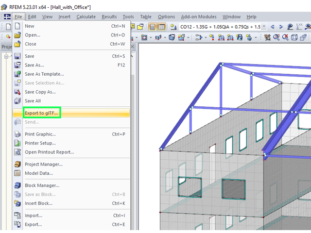
RFEM and RSTAB models can be saved as 3D glTF models (*.glb and *.glTF formats). View the models in 3D in detail with a 3D viewer from Google or Babylon. Take your VR glasses, such as Oculus, to "walk" through the structure.
You can integrate the 3D glTF models into your own websites using JavaScript according to these instructions (as on the Dlubal website Models to Download).
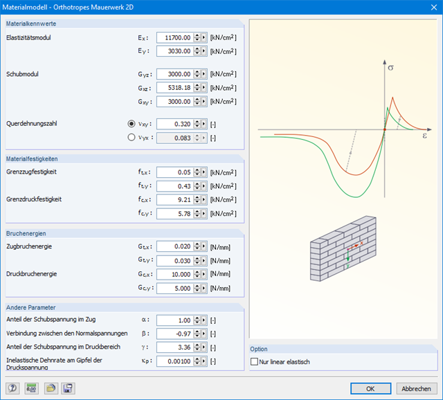
The material model Orthotropic Masonry 2D is an elastoplastic model that additionally allows softening of the material, which can be different in the local x- and y-directions of a surface. The material model is suitable for (unreinforced) masonry walls with in-plane loads.
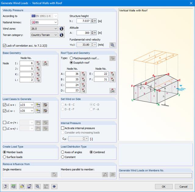
Wind loads can be automatically generated as member loads or area loads on the following structural components (optional with internal pressure for open buildings):
- Vertical walls
- Flat roofs
- Monopitch roofs
- Duopitch/troughed roofs
- Vertical walls with roof
The following standards are available:
-
 EN 1991-1-3 (incl. National Annexes)
 -
 DIN 1055-4
 -
 CTE DB-SE-AE
 -
 ASCE/SEI 7-16

To test the program before purchasing an RFEM or RSTAB license, you can download the free 90-day trial version. This will allow you to test the full version of the program without any limitations.
Download Trial Versions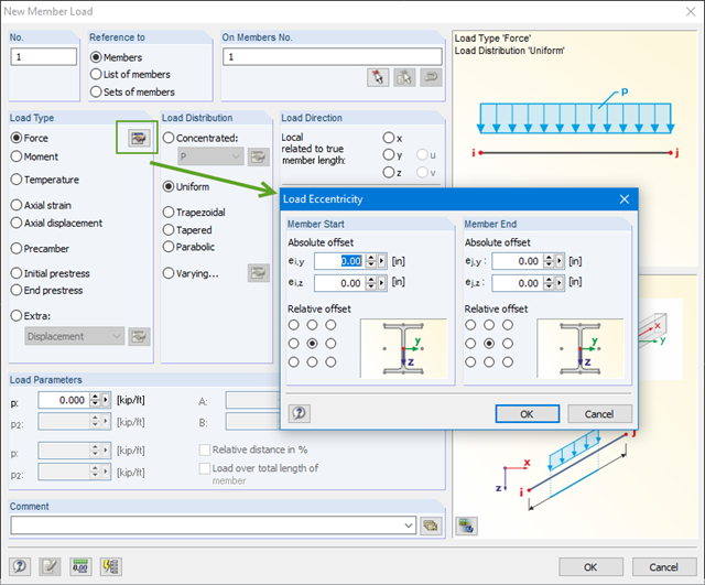
You can define eccentricities for member loads of the load type 'Force'. You can apply the load eccentricities by means of an absolute or relative offset.
We recommend using the large deformation analysis to consider all effects of eccentric loads.

The introductory examples and tutorials for RFEM 5 and RSTAB 8 will help you to get started with the program. Step by step, you will become familiar with the most important features. You can download the documents in PDF format.
Introductory Example for RFEM 5 (PDF) Tutorial for RFEM 5 (PDF) Introductory Example for RSTAB 8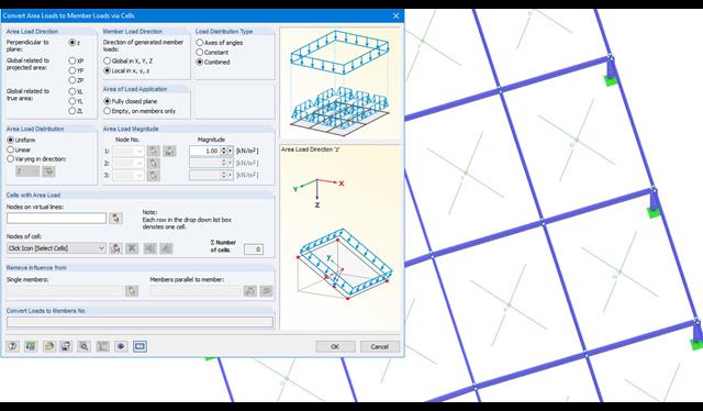
Area loads can be automatically converted into member or line loads. There are 3 options available for this:
- Generate Member Loads from Area Load via Plane
- Member loads from area loads via cells
- Line loads from surface loads on openings
In the case of member loads from area loads, a plane has to be defined via corner nodes or cells have to be selected in the graphic. The area load can either be applied to the entire surface or only the effective or projected surface of the members.
For the 'Line Loads from Area Loads on Openings' function, the corresponding openings are selected.
Online Manual RFEM | Member Loads from Area Loads via Plane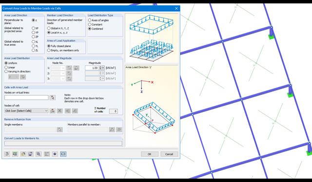
Area loads can be automatically converted into member loads. There are 2 options available for this:
- Generate Member Loads from Area Load via Plane
- Member loads from area loads via cells
Depending on the selected option, you either have to define a plane via corner nodes or select cells in the graphic. The area load can either be applied to the entire surface or only the effective or projected surface of the members.
Online Manual RFEM | Member Loads from Area Loads via Plane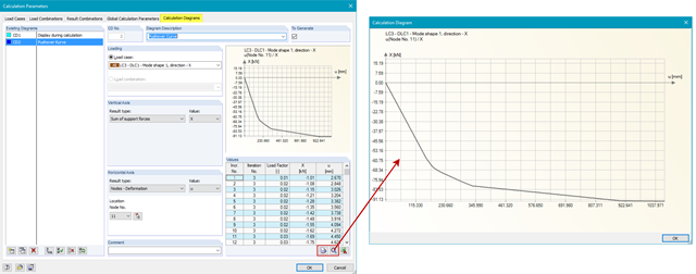
In RFEM, it is possible to determine pushover curves (also called capacity curves) and export them to Excel.
With the RF-DYNAM Pro - Equivalent Loads add-on module, it is possible to generate load distribution automatically in accordance with a mode shape and export it as a load case to RFEM.
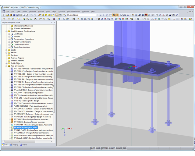
At first, the governing joint designs are arranged in groups and displayed with the basic geometry of the joint in the first result window. In the other result tables, you can see all fundamental design details such as the load-carrying capacity of anchors, stresses in welds, and others.
Dimensions, material specifications, and welds that are important for the construction of the connection are visible immediately and can be printed out. It is possible to visualize the connections in RF-/JOINTS Steel - Column Base or in the RFEM/RSTAB model.
All graphics can be included in the RFEM/RSTAB printout report or printed directly. Due to the scaled output, an optimal visual check is possible as early as in the design phase.
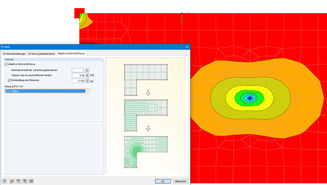
With this function, it is possible to refine the FE mesh on surfaces automatically. The mesh refinement is gradual. In each step, the FE mesh is recreated based on an error comparison of the results in the previous calculation step. The numerical error is evaluated from the results of surface elements and is based on the energy formulation of Zienkiewicz-Zhu.
The error evaluation is carried out for a linear static analysis. We select a load case (or load combination) for which the FE mesh is generated. The FE mesh is then used for all calculations.
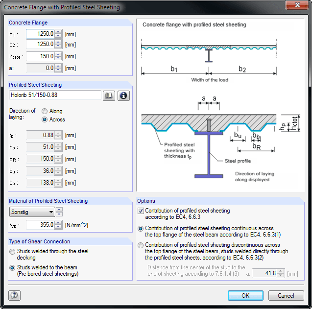
When entering the structural model, you can define single-span and continuous beams with or without cantilevers. Furthermore, it is possible to specify different span lengths with definable boundary conditions (supports, releases) as well as any construction support and moment release in the construction stage. For a complete cross-section, you can create typical composite beam sections on the basis of steel girders (I-sections) with solid concrete flanges, precast plates, trapezoidal sheets, or tapered solid ceilings.
It is also possible to grade cross-sections by means of beam lengths, optionally with concrete encasement. Illustrative figures facilitate the entry of additional transverse reinforcements for trapezoidal sheeting, profile stiffeners, and angled or circular openings in the web. The self-weight is applied automatically when entering loads. In addition, it is possible to consider fixed and variable loads by specifying the concrete age at the beginning of loading for creeping, and to define single, uniform, and trapezoidal loads freely. COMPOSITE-BEAM automatically creates a load combination based on the data of individual load cases.
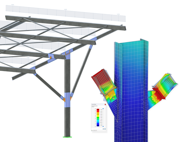
Steel bolted connections with gusset plates on the canopy structure.
Download the structural analysis model and open it with the finite element program RFEM 6 using Steel Joints Add-on.
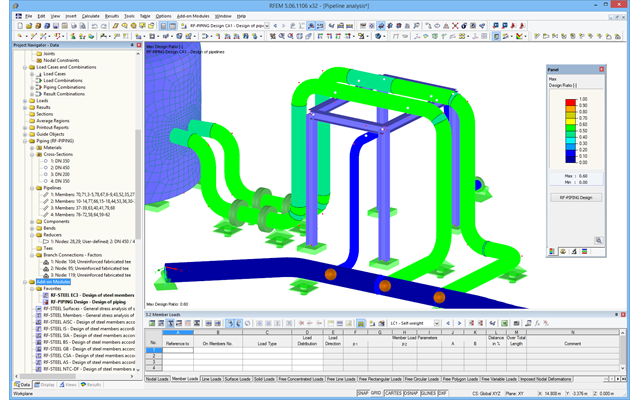
After modeling piping systems in RFEM using RF‑PIPING and defining loads as well as load and result combinations, you can carry out pipe stress analysis in the RF‑PIPING Design add‑on module.
You can select all or only some pipelines and loads, load or result combinations for piping design. The material library provides various materials according to EN 13480‑3, ASME B31.1‑2012, and ASME B31.3‑2012 standards.
After the calculation, the results are displayed in clearly arranged windows; for example, by cross‑section, by pipeline, or by members. You can also display the design ratio graphically on the entire model in RFEM. This way, you can quickly recognize critical or oversized areas of the cross-section.
In addition to the input and result data, including design details displayed in tables, you can add all graphics into the printout report. This way, comprehensible and clearly arranged documentation is guaranteed. You can select the report contents and extent specifically for the individual designs.
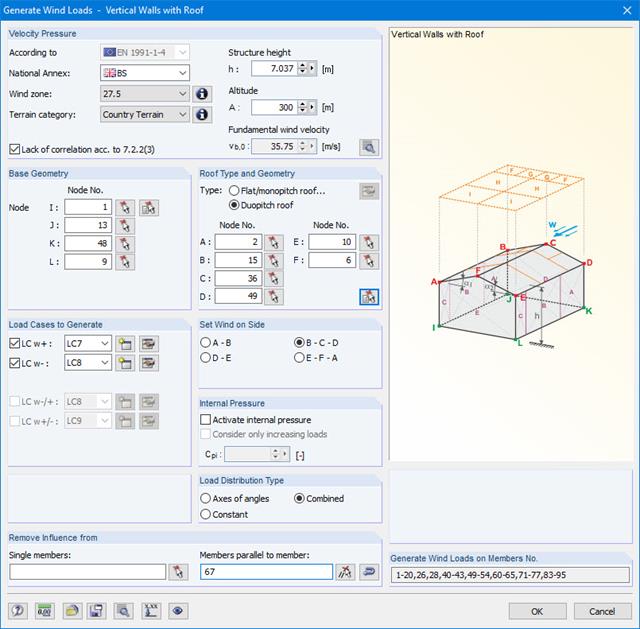
Wind loads can be automatically generated as member loads on the following structural components (optional with internal pressure for open buildings):
- Vertical walls
- Flat roofs
- Monopitch roofs
- Duopitch/troughed roofs
- Vertical walls with roof
The following standards are available:
-
EN 1991-1-3 (incl. National Annexes)
-
DIN 1055-4
-
CTE DB-SE-AE
-
ASCE/SEI 7-16
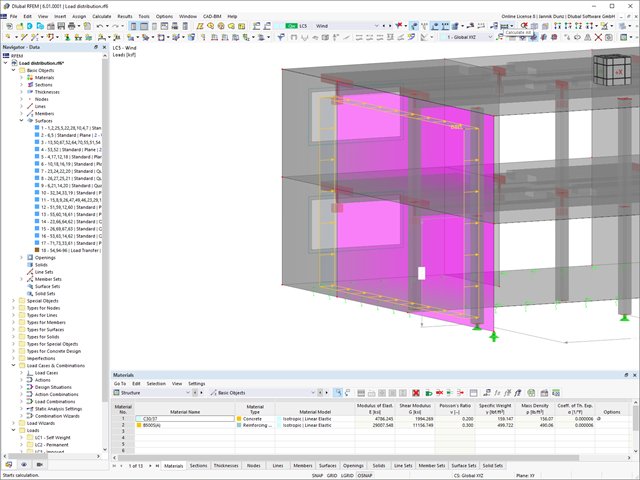
Keep an eye on all surfaces. A surface with the "Load Transfer" stiffness type has no structural effect. You can use it to consider the loads from surfaces that have not been modeled, for example, facade structures, glass surfaces, trapezoidal roof sections, and so on.
Go to Explanatory Video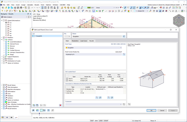
Do you want your structures to remain upright even in wind and snow? Then rely on the load wizards for plate and frame structures. You can now generate wind loads according to EN 1991‑1‑4 and snow loads according to EN 1991‑1‑3 (as well as other international standards). The load cases are generated depending on the roof shape.
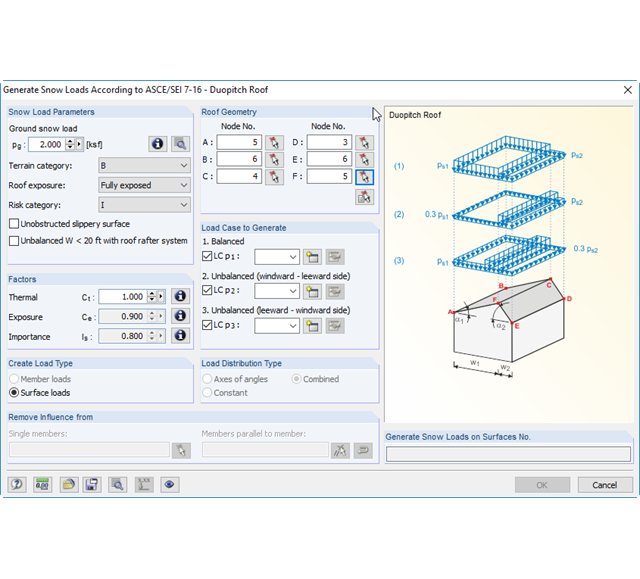
There are load generators available for beam structures, creating snow loads according to ASCE/SEI 7-10. The load cases are generated depending on the roof shape. Another generator creates coating loads (ice). You can save recurring load combinations as templates.
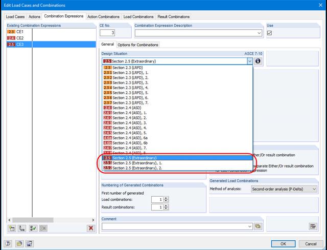
When you select the design situation 'Accidental', accidental actions such as earthquake, explosion loads, collisions, and others are automatically taken into account. When applying German standards, you can automatically consider the 'North German Plain' by selecting the design situation 'Accidental - Snow'.
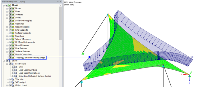
With the activated option 'Topology on Form-Finding Form' in Project Navigator - Display, the model display is optimized based on the form-finding geometry. For example, the loads are displayed in relation to the deformed system.
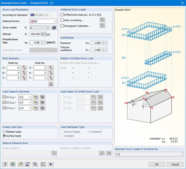
The snow load generator can generate snow loads as member loads or surface loads.
Additional snow loads such as drifted snow loads, snow overhangs, and snow guards can be taken into account as well.
The following standards are available:
-
EN 1991-1-3 (incl. National Annexes)
-
DIN 1055-5
-
CTE DB-SE-AE
-
ASCE/SEI 7-16
Always keep an eye on your results. In addition to the resulting load cases in RFEM or RSTAB (see below), the results from the aerodynamics analysis in RWIND 2 represent the flow problem as a whole:
- Pressure on structure surface
- Pressure field about structure geometry
- Velocity field about structure geometry
- Velocity vectors about structure geometry
- Flow lines about structure geometry
- Forces on member-shaped structures that were originally generated from member elements
- Convergence diagram
- Direction and size of the flow resistance of the defined structures
These results are displayed in the RWIND 2 environment and evaluated graphically. The flow results around the structure geometry in the overall display are rather confusing, but the program has a solution for this. In order to present clearly arranged results, freely movable section planes are displayed for the separate display of the 'solid results' in a plane. Accordingly, for the 3D branched streamline result, the program presents you an animated display in the form of moving lines or particles in addition to the static one. This option helps to represent the wind flow as a dynamic effect.
You can export all results as a picture or, especially for the animated results, as a video.
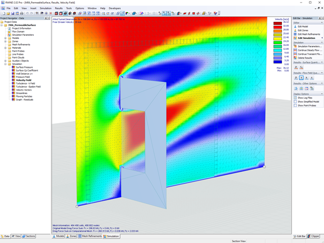
Use RWIND 2 Pro to easily apply a permeability to a surface. All you need is the definition of
- the Darcy coefficient D,
- the inertial coefficient I, and
- the length of the porous medium in the direction of flow L,
to define a pressure boundary condition between the front and back of a porous zone. Due to this setting, you obtain the flow through this zone with a two-part result display on both sides of the zone area.
But that's not all. Furthermore, the generation of a simplified model recognizes permeable zones and takes into account the corresponding openings in the model coating. Can you waive an elaborate geometric modeling of the porous element? Understandable – we have good news for you then! With a pure definition of the permeability parameters, you can avoid complex geometric modeling of the porous element. Use this feature to simulate permeable scaffolding, dust curtains, mesh structures, and so on.
More Information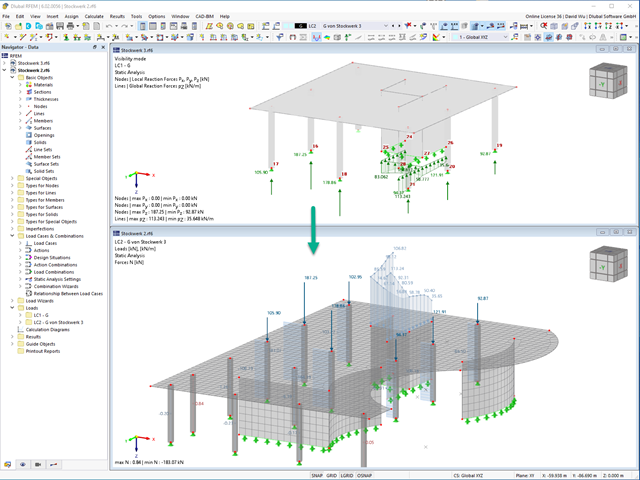
This function provides you with the option to adopt reaction forces from other models as nodal and line loads.
The option not only transfers the reaction load as an action, but digitally couples the support load of the original model with the load size of the target object. The subsequent changes in the original model are automatically adopted in the target model.
This technology supports the concept of positional statics and allows you to digitally connect the individual positions of the same Dlubal Center project.
Go to Explanatory Video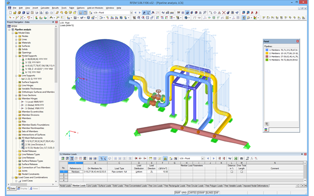
After activating the RF‑PIPING add‑on module, a new toolbar is available in RFEM and the project navigator and tables are extended. The piping system is now modeled in the same way as the members. Pipe bends are defined simultaneously by tangents (straight pipe sections) and radius. Thus, it is easy to subsequently change bend parameters.
It is also possible to extend the piping subsequently by defining special components (expansion joints, valves, and others). The implemented libraries of structural components facilitate the definition.
Continuous pipe sections are defined as sets of piping systems.
For piping loads, member loads are assigned to the respective load cases. The combination of loads is included in piping load combinations and result combinations.
After the calculation, you can display deformations, member internal forces, and support forces graphically or in tables.
Pipe stress analysis according to standards can then be performed in the RF‑PIPING Design add‑on module. You only need to select the relevant sets of piping systems and load situations.
- Calculation of transient incompressible turbulent wind flow with the BlueDyMSolver solver
- LES SpalartAllmarasDDES turbulence model
- Consideration of stationary solution as initial state for transient calculation
- Automatic determination of analysis period and time steps
- Use of intermediate results during the calculation
- Organized display of time-varying results via time step units
- Diagram of drag force and point probe results over analysis time
- Display of line probe results for any time steps in a diagram
- Freely adjustable wind permeability for surfaces (Go to Product Feature)
- Structure generator for typical geometries with loading and combinations
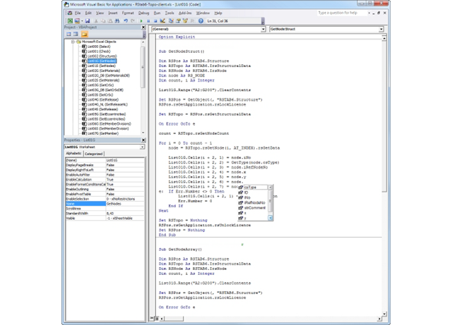
- Importing and exporting data from spreadsheet programs such as MS Excel and MS Access
- Connection to various programs compatible with COM, for example, B. CAD systems
- Customized pre- and postprocessing modules
- Processing and results of data in user-defined formats
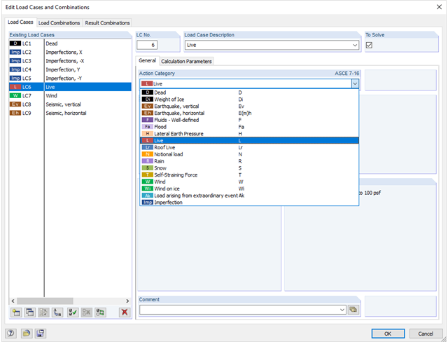
In the "Edit Load Cases and Combinations" dialog box, you can create and edit load cases as well as generate action, load, and result combinations. It is possible to assign various action types to the individual load cases in accordance with the selected standard. If several loads have been assigned to one action type, they can act simultaneously or alternatively (for example, wind from the left or right).
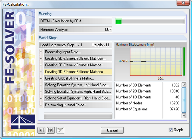
The equation solver includes an optimized FE mesh generator and supports the latest multi-core processor and 64-bit technology. It enables parallel calculations of linear load cases and load combinations using several processors without additional demands on the RAM: The stiffness matrix only has to be created once. The 64-bit technology and the enhanced RAM options allow for calculation of complex structural systems using the fast and direct equation solver.
The development of the deformation is displayed in a diagram during the calculation. This way, you can easily evaluate the convergence behavior.
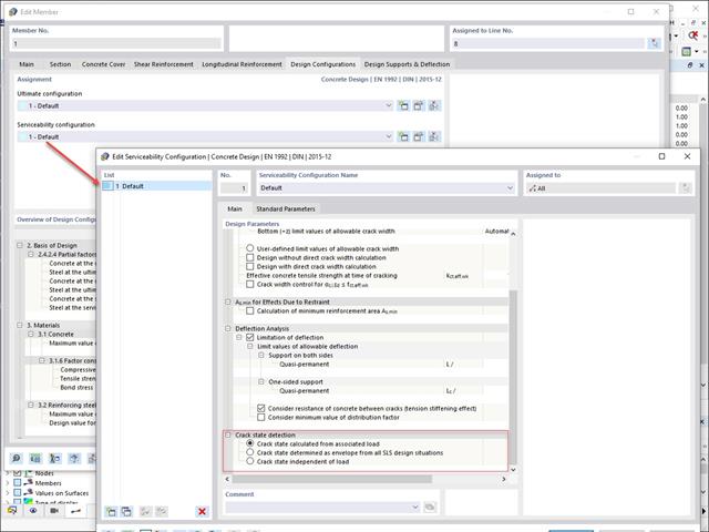
Various design parameters of the cross-sections can be adjusted in the serviceability limit state configuration. The applied cross-section condition for the deformation and crack width analysis can be controlled there.
For this, the following settings can be activated:
- Crack state calculated from associated load
- Crack state determined as an envelope from all SLS design situations
- Cracked state of cross-section - independent of load