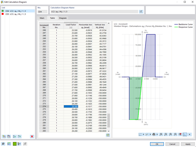
For calculation diagrams, you can use the "2D | Hinge" diagram type. These hinge diagrams show the hinge response of load situations for nonlinear hinges.
For calculations with several load situations, such as the case with the pushover analysis and time history analysis, you can evaluate the hinge condition in each load step.
- Analysis of time diagrams and accelerograms (acceleration-time diagrams exciting the supports of a structure)
- Combination of user-defined time diagrams with nodal, member, and surface loads, as well as free and generated loads
- Combination of several independent excitation functions
- Linear implicit Newmark analysis or modal analysis in time history
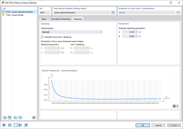
- Structural damping using Raleigh damping coefficients or Lehr's damping value
- Graphical display of results in calculation diagrams
- Result display in individual time steps or as an envelope during the entire time period
- Extensive library of seismic events (accelerograms)
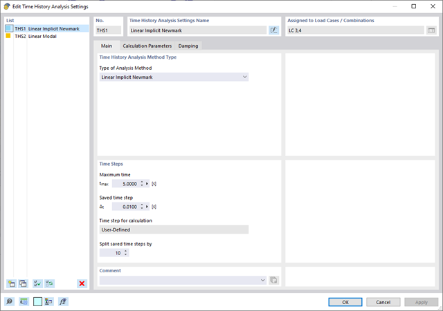
The time history analysis is performed with the modal analysis or the linear implicit Newmark analysis. The time history analysis in this add-on is limited to linear structural systems. Although the modal analysis represents a fast algorithm, it is necessary to use a certain number of eigenvalues to ensure the required accuracy of results.
The implicit Newmark analysis is a very precise method, independent of the number of eigenvalues used, but requires sufficient small time steps for the calculation.
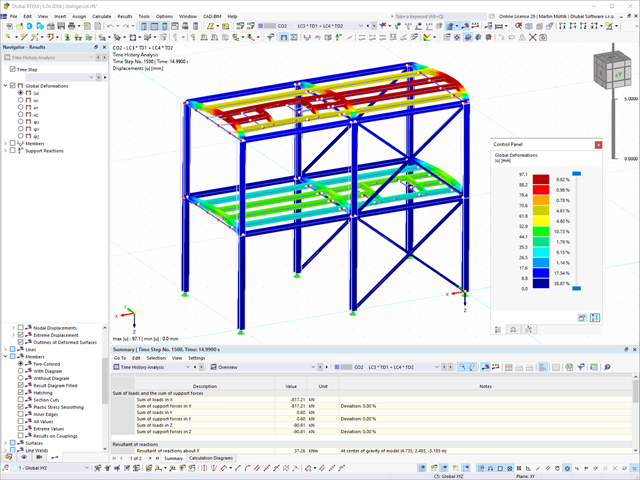
As soon as the program has completed the calculation, the summary of the results is listed. All result windows are integrated in the main program RFEM/RSTAB. You will find all the results arranged in tables; they can be displayed for each individual time step or as an envelope, and you also have the option of displaying the results graphically as well as animating them.
The results from the time history analysis can be displayed in the calculation diagrams. All the results are shown as a function of time. You can export the numeric values to MS Excel.
All result tables and graphics are part of the RFEM/RSTAB printout report. In this way, you can ensure clearly arranged documentation. You can also export the tables to MS Excel.
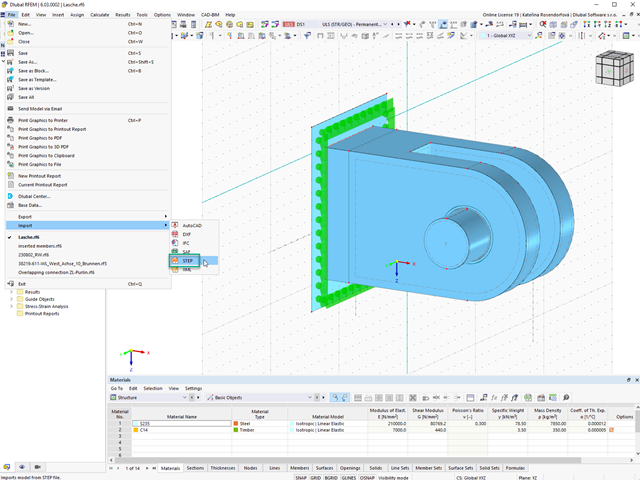
You can import STEP files into RFEM 6. The data are directly converted into the native RFEM model data.
STEP is an interface standard initiated by ISO (ISO 10303). In the geometry description, all shapes relevant for RFEM (line, surface, and solid models) can be integrated by the CAD data models.
Note: This format is not to be confused with DSTV interfaces, which also use the file extension *.stp.
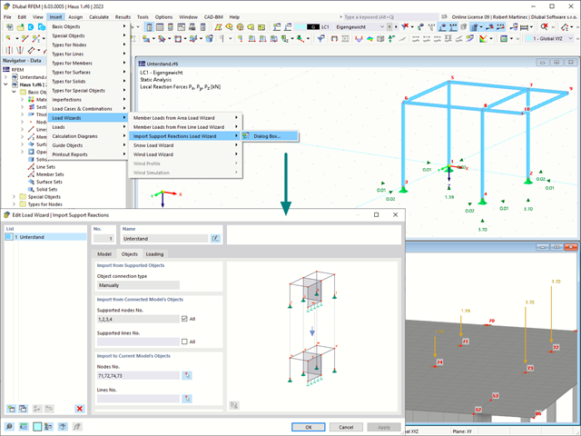
Use the "Import Support Reactions" Load Wizard in RFEM 6 and RSTAB 9 to easily transfer reaction forces from other models. The wizard allows you to connect all or several nodal and line loads of different models with each other in a few steps.
The load transfer from load cases and load combinations can be carried out automatically or manually. It's necessary that the models are saved in the same Dlubal Center project.
The "Import Support Reactions" load wizard supports the concept of positional statics and allows you to digitally connect the individual positions.
Go to Explanatory Video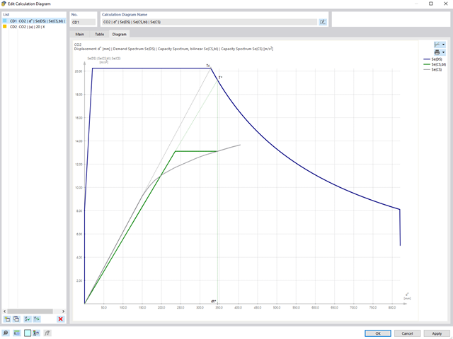
During the calculation, the selected horizontal load is increased in load steps. A static nonlinear analysis is carried out for each load step until reaching the specified limit condition.
The results of the pushover analysis are extensive. On one hand, the structure is analyzed for its deformation behavior. This can be represented by a force-deformation line of the system (a capacity curve). On the other hand, the response spectrum effect can be displayed in the ADRS display (Acceleration-Displacement Response Spectrum). The target displacement is automatically determined in the program based on these two results. The process can be evaluated graphically and in tables.
The individual acceptance criteria can then be graphically evaluated and assessed (for the next load step of the target displacement, but also for all other load steps). The results of the static analysis are also available for the individual load steps.
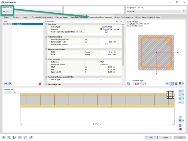
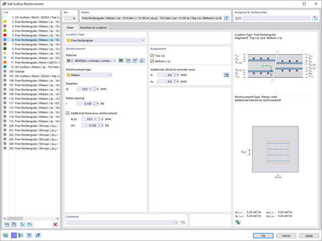
Utilize this time-saving step! This feature allows you to define or edit the member reinforcement for several members or member sets at the same time.
Go to Explanatory Video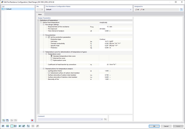
The component temperature to be applied at the design time is determined automatically. You can adjust the coefficients used to determine the temperature. In this step, it is best for you to also select the hot-dip galvanizing. According to the DASt Guideline 027 "Determination of Component Temperature of Hot-Dip Galvanized Steel Components in Case of Fire", a lower emissivity of the steel surface is applied up to a limit temperature. Overall, this gives you a lower temperature for the thus more favorable fire resistance design.
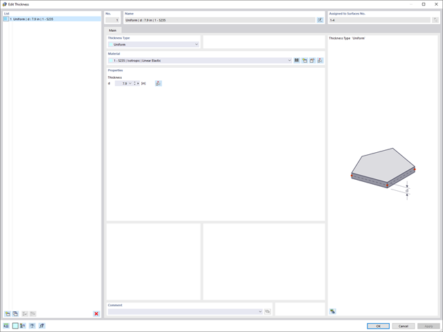
If you want to describe surface thicknesses, you can now use a new thickness object. It can be used for several surfaces. If you modify the thickness of this object, all assigned surface thicknesses are adjusted accordingly in one step.
.jpg?mw=640&hash=26a7c7d3eca4bc6f129e08b373eac4f2314109ba)
Take your structural design one step further. RFEM 6 and RSTAB 9 support now a new file format for structural design, Structural Analysis Format (SAF). For this, both programs allow for the import as well as the export. SAF is a file format based on MS Excel, intended to facilitate the exchange of structural analysis models between different software applications.
- Calculation of transient incompressible turbulent wind flow with the BlueDyMSolver solver
- LES SpalartAllmarasDDES turbulence model
- Consideration of stationary solution as initial state for transient calculation
- Automatic determination of analysis period and time steps
- Use of intermediate results during the calculation
- Organized display of time-varying results via time step units
- Diagram of drag force and point probe results over analysis time
- Display of line probe results for any time steps in a diagram
- Freely adjustable wind permeability for surfaces (Go to Product Feature)
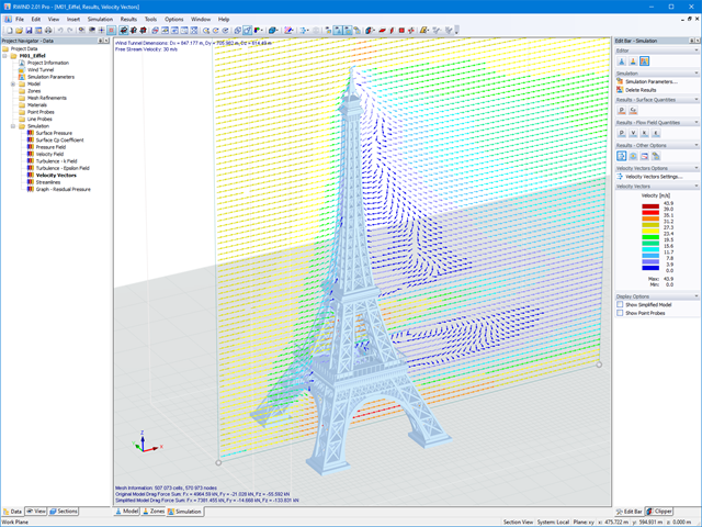
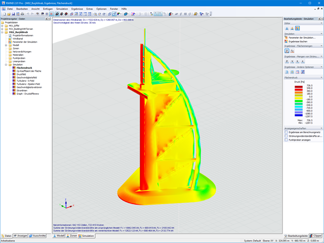
RWIND Basic uses a numerical CFD model (Computational Fluid Dynamics) to simulate wind flows around your objects using a digital wind tunnel. The simulation process determines specific wind loads acting on your model surfaces from the flow result around the model.
A 3D volume mesh is responsible for the simulation itself. For this, RWIND Basic performs an automatic meshing on the basis of freely definable control parameters. For the calculation of wind flows, RWIND Basic provides you with a stationary solve and RWIND Pro provides a transient solver for incompressible turbulent flows. Surface pressures resulting from the flow results are extrapolated onto the model for each time step.
When starting the analysis in the RFEM or RSTAB application, you trigger a batch process. It places all member, surface, and solid definitions of the model rotated with all relevant coefficients in the numerical wind tunnel of RWIND Basic. Furthermore, it starts the CFD analysis, and returns the resulting surface pressures for a selected time step as FE mesh nodal loads or member loads into the respective load cases of RFEM or RSTAB.
These load cases which contain RWIND Basic loads can then be calculated. Moreover, you can combine them with other loads in load and result combinations.

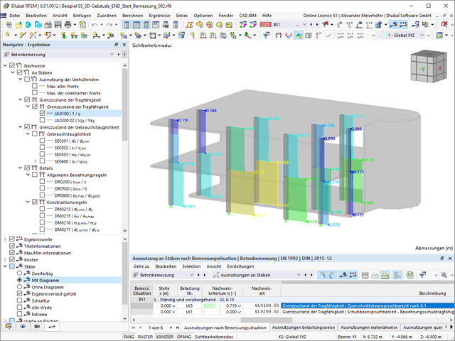
Compared to the RF‑/STABILITY (RFEM 5) and RSBUCK (RSTAB 8) add-on modules, the following new features have been added to the Structure Stability add-on for RFEM 6 / RSTAB 9:
- Activation as a property of a load case or a load combination
- Automated activation of the stability calculation via combination wizards for several load situations in one step
- Incremental load increase with user-defined termination criteria
- Modification of the mode shape normalization without recalculation
- Result tables with filter option

- 002109
- General
- Optimization & Cost / CO2 Emission Estimation for RFEM 6
- Optimization & Cost / CO2 Emission Estimation for RSTAB 9
Did you know? The structural optimization in the programs RFEM and RSTAB is a completion of the parametric input. It is a parallel process beside the actual model calculation with all its regular calculation and design definitions. The add-on assumes that your model or block is built with a parametric context and is controlled in its entirety by global control parameters of the "optimization" type. Therefore, these control parameters have a lower and upper limit and a step size to delimit the optimization range. If you want to find optimal values for the control parameters, you have to specify an optimization criterion (for example, minimum weight) with the selection of an optimization method (for example, particle swarm optimization).
You can already find the cost and CO2 emission estimation in the material definitions. You can activate both options individually in each material definition. The estimation is based on a unit for unit cost or unit emission for members, surfaces, and solids. In this case, you can select whether to specify the units by weight, volume, or area.
The standards already specify the approximation methods (for example, deformation calculation according to EN 1992‑1‑1, 7.4.3, or ACI 318‑19, 24.3.2.5) that you need for your deformation calculation. In this case, the so-called effective stiffnesses are calculated in the finite elements in accordance with the existing limit state with / without cracks. You can then use these effective stiffnesses to determine the deformations by means of another FEM calculation.
Consider a reinforced concrete cross-section for the calculation of the effective stiffnesses of the finite elements. Based on the internal forces determined for the serviceability limit state in RFEM, you can classify the reinforced concrete cross-section as "cracked" or "uncracked". Do you consider the effect of the concrete between the cracks? In this case, this is done by means of a distribution coefficient (for example, according to EN 1992‑1‑1, Eq. 7.19, or ACI 318‑19, 24.3.2.5). You can assume the material behavior for the concrete to be linear-elastic in the compression and tension zone until reaching the concrete tensile strength. This procedure is sufficiently precise for the serviceability limit state.
When determining the effective stiffnesses, you can take into accout the creep and shrinkage at the "cross-section level." You don't need to consider the influence of shrinkage and creep in statically indeterminate systems in this approximation method (for example, tensile forces from shrinkage strain in systems restrained on all sides are not determined and have to be considered separately). In summary, the deformation calculation is carried out in two steps:
- Calculation of effective stiffnesses of the reinforced concrete cross-section assuming linear-elastic conditions
- Calculation of the deformation using the effective stiffnesses with FEM
Dlubal Software makes many of your work steps easier to support you. Thus, the surfaces, members, member sets, materials, surface thicknesses, and sections defined in RFEM/RSTAB are preset to facilitate the data input. You can use the [Select] function at many places of the program to select the elements graphically. Furthermore, you have an access to the global material and cross-section libraries.
You can group surfaces or members into "Configurations", each with different design parameters. This way, it is possible for you to efficiently calculate design alternatives with different boundary conditions or modified cross-sections, for example. You will be amazed how much faster everything works with RFEM/RSTAB.
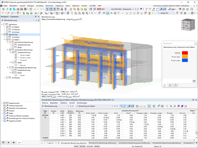
Do you want to perform the bending failure design? To do this, analyze the governing locations of the column for axial forces and moments. For the shear resistance design, you can also consider the locations with extreme values of shear forces. During the calculation, you determine whether a standard design is sufficient or whether the column with the moments has to be designed according to the second-order theory. You can then determine these moments using the previously entered specifications. The calculation is divided into three parts:
- Load-independent calculation steps
- Iterative determination of governing loading taking into account a varying required reinforcement
- Safety determination of all acting internal forces, including the designed reinforcement
After a successful calculation, the results are displayed in clearly arranged tables. Each intermediate value is absolutely traceable, making the design checks transparent.

- 3D incompressible wind flow analysis with OpenFOAM® software package
- Direct model import from RFEM or RSTAB including neighboring and terrain models (3DS, IFC, STEP files)
- Model design via STL or VTP files independent of RFEM or RSTAB
- Simple model changes using Drag and Drop and graphical adjustment assistance
- Automatic corrections of the model topology with shrink wrap networks
- Option to add objects from the environment (buildings, terrain ...)
- Wind load determined over the height of the building, depending on standard-specific parameters (velocity, turbulence intensity)
- K-epsilon and K-omega turbulence models
- Automatic mesh generation adjusted to the selected depth of detail
- Parallel calculation with optimal utilization of the capacity of multicore computers
- Results in just minutes for low-resolution simulations (up to 1 million cells)
- Results within a few hours for simulations with medium/high resolution (1‑10 million cells)
- Graphical display of results on the Clipper/Slicer planes (scalar and vector fields)
- Graphical display of streamlines
- Streamline animation (optional video creation)
- Definition of point and line probes
- Display of aerodynamic pressure coefficients
- Graphical display of turbulence properties in the wind field
- Optional meshing using the boundary layer option for the area near the model surface
- Consideration of rough model surfaces possible
- Optional use of a seond-order numerical Order
- Multilingual user interface (for example, German, English, Spanish, French)
- Documentation possible in the RFEM and RSTAB printout report
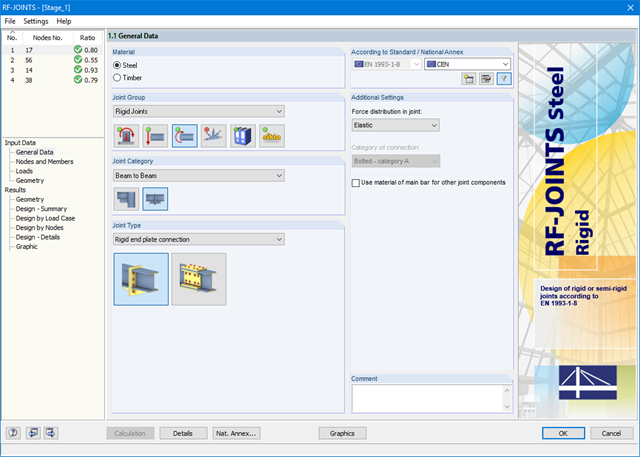
After starting the module, the joint group (rigid joints) is selected first, followed by joint category and joint type (rigid end plate connection or rigid splice plate connection). The nodes to be designed are then selected from the RFEM/RSTAB model. RF-/JOINTS Steel - Rigid automatically recognizes the joint members and determines from its location whether they are columns or beams. The user can intervene here.
If certain members are to be excluded from the calculation, they can be deactivated. Structurally similar connections can be designed for several nodes at the same time. Loads require selection of the governing load cases, load combinations, or result combinations. Alternatively, you can enter the cross‑section and load data manually. In the last input window, the connection is configured step by step.
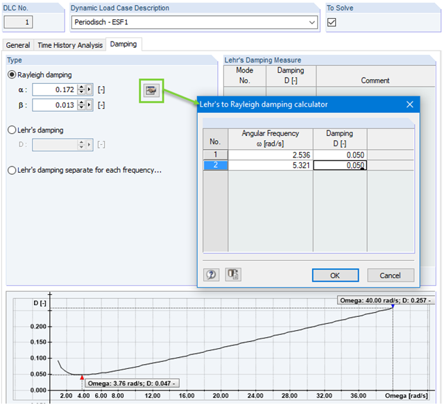
Calculation with consideration of a damping ratio (or Lehr's damping) is not possible in the direct time step integrations. Instead, the Rayleigh damping coefficients must be specified by the user.
In technical literature, the given damping ratio for specific construction forms is, in many cases, only a rough approximation of the real damping ratios. In RF-/DYNAM Pro - Forced Vibrations, it is possible to use the value of the damping ratio to determine the Rayleigh damping. This may occur at one or two natural angular frequencies defined by the user.
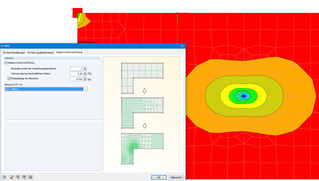
With this function, it is possible to refine the FE mesh on surfaces automatically. The mesh refinement is gradual. In each step, the FE mesh is recreated based on an error comparison of the results in the previous calculation step. The numerical error is evaluated from the results of surface elements and is based on the energy formulation of Zienkiewicz-Zhu.
The error evaluation is carried out for a linear static analysis. We select a load case (or load combination) for which the FE mesh is generated. The FE mesh is then used for all calculations.
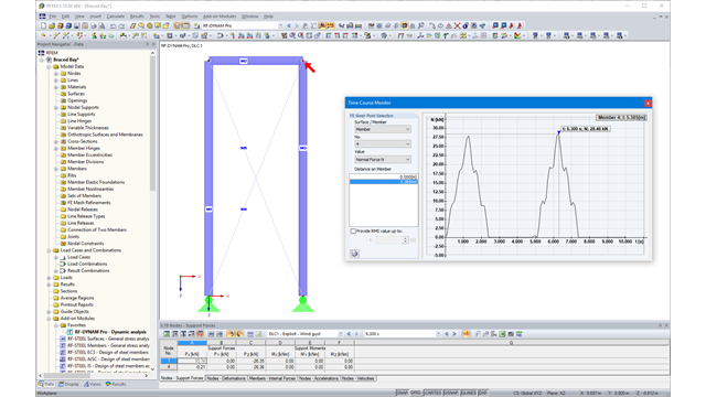
Due to the integration of RF‑/DYNAM Pro in RFEM or RSTAB, you can incorporate numeric and graphic results from RF‑/DYNAM Pro - Nonlinear Time History to the global printout report. Also, all RFEM and RSTAB options are available for a graphical visualization. The results of the time history analysis are displayed in a time history diagram.
The results are displayed as a function of time and the numerical values can be exported to MS Excel. Result combinations can be exported, either as a result of a single time step or the most unfavorable results of all time steps are filtered out.
Calculation in RFEM
The nonlinear time history analysis is performed with the implicit Newmark analysis or the explicit analysis. Both are direct time integration methods. The implicit analysis requires small time steps to provide precise results. The explicit analysis determines the required time step automatically to provide the stability to the solution. The explicit analysis is suitable for the analysis of short excitations, such as impulse excitation, or an explosion.
Calculation in RSTAB
The nonlinear time history analysis is performed with the explicit analysis. This is a direct time integration method and determines the required time step automatically in order to provide the solution stability.
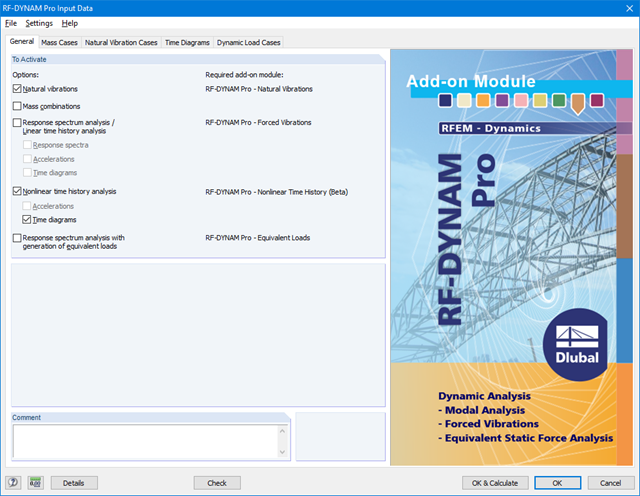
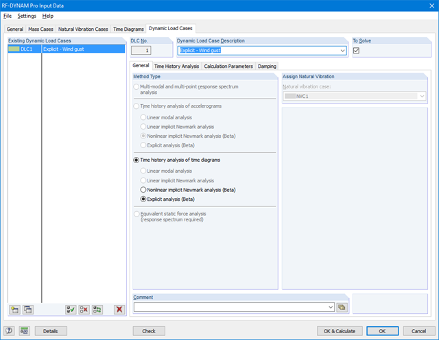
RF-/DYNAM Pro - Nonlinear Time History is integrated in the structure of RF‑/DYNAM Pro - Forced Vibrations and extended by two nonlinear analysis methods (one nonlinear analysis in RSTAB).
Force-time diagrams can be entered as transient, periodic, or as a function of time. Dynamic load cases combine the time diagrams with the static load cases, which provides high flexibility. Furthermore, it is possible to define time steps for the calculation, structural damping, and export options in the dynamic load cases.
.png?mw=640&hash=8cfd0c4bd093c03de543d147ffbf6f5c9250634a)
- User-defined time diagrams as a function of time, in tabular form, or as harmonic loads
- Combination of the time diagrams with RFEM/RSTAB load cases or combinations (enables definition of nodal, member, and surface loads, as well as free and generated loads varying over time)
- Combination of several independent excitation functions
- Nonlinear time history analysis with the implicit Newmark analysis (RFEM only) or the explicit analysis
- Structural damping using Rayleigh damping coefficients or Lehr's damping
- Direct import of initial deformations from a load case or combination (RFEM only)
- Stiffness modifications as initial conditions; for example, axial force effect, deactivated members (RSTAB only)
- Graphical display of results in a time history diagram
- Export of results in user-defined time steps or as an envelope
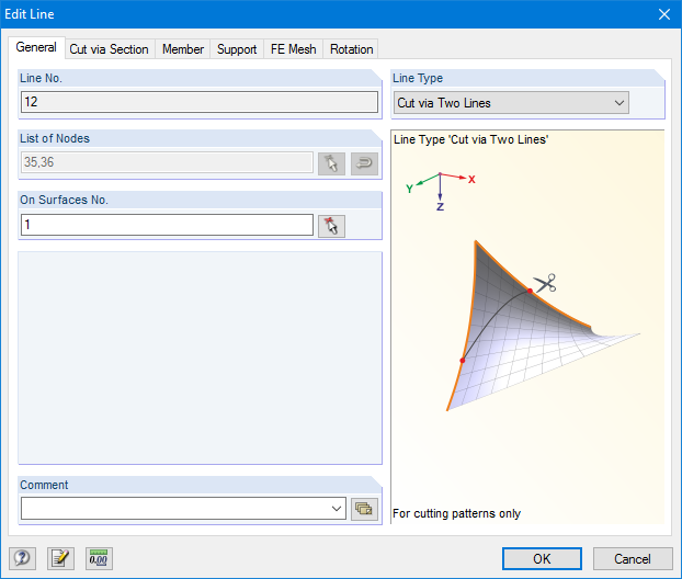
RF-CUTTING-PATTERN is activated by selecting the respective option in the Options tab in General Data of any RFEM model. After activating the add‑on module, a new object, "Cutting Patterns", is displayed under Model Data. If the membrane surface distribution for cutting in the basic position is too large, you can divide the surface by cutting lines (line types "Cut via Two Lines" or "Cut via Section") in the corresponding partial strips.
Then you can define the individual entries for each cutting pattern using the "Cutting Pattern" object. Here you can set boundary lines, compensations, and allowances.
Steps of the working sequence:
- Creation of cutting lines
- Creation of the pattern by selecting its boundary lines or using a semi‑automatic generator
- Free selection of warp and weft orientation by entering an angle
- Application of compensation values
- Optional definition of different compensations for boundary lines
- Different allowances (welding, boundary line)
- Preliminary representation of the cutting pattern in the graphic window at the side without starting the main nonlinear calculation
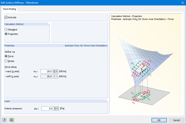
The form-finding function can be activated in the General Data dialog box, Options tab. Prestresses (or geometrical requirements for members) can be defined in the parameters for surfaces and members. The form‑finding process is performed by calculation of an RF‑FORM‑FINDING case.
Steps of the working sequence:
- Creation of a model in RFEM (surfaces, beams, cables, supports, material definition, and so on)
- Setting of required prestress for membranes and force or length/sag for members (for example, cable)
- Optional consideration of other loads for the form-finding process in special form‑finding load cases (self‑weight, pressure, steel node weight, and so on)
- Setting of loads and load combinations for further structural analyses
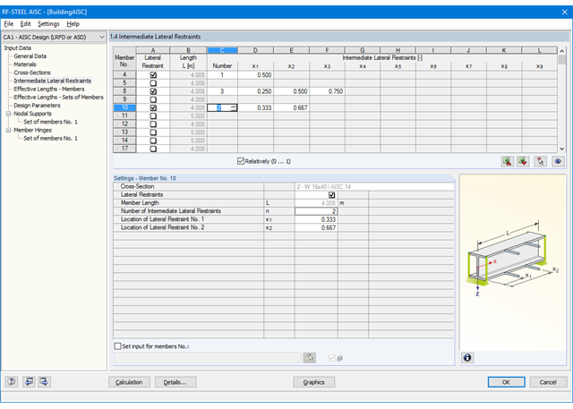
First, it is necessary to decide whether to perform design according to ASD or LRFD. Then, you can enter the load cases, load combinations, and result combinations to be designed. Load combinations according to ASCE 7 can be generated either manually or automatically in RFEM/RSTAB.
In the next steps, you can adjust presettings of lateral intermediate supports, effective lengths, and other standard-specific design parameters, such as the modification factor Cb for lateral-torsional buckling or the shear lag factor. In the case of continuous members, it is possible to define individual support conditions and eccentricities of each intermediate node of single members. A special FEA tool determines critical loads and moments required for the stability analysis.
In connection with RFEM/RSTAB, it is possible to apply the Direct Analysis Method taking into account the influence of the general calculation according to the second-order analysis. In this way, you avoid using special enlargement factors.