104 Wyniki
Wyświetl wyniki:
Sortuj według:

Tabela wyników modelu budynku 'Wyniki według kondygnacji' przedstawia środek ciężkości przypadków obciążeń i kombinacji obciążeń. Oprócz obciążenia stałego uwzględniane są również obciążenia pionowe odpowiednich przypadków obciążeń i kombinacji obciążeń.
W celu wyświetlenia środka ciężkości z uwzględnieniem wybranego obciążenia można również użyć okna dialogowego 'Środek ciężkości oraz Informacje o wybranych obiektach.

W rozszerzeniu Analiza geotechniczna dostępny jest wysokiej jakości model materiałowy "Zmodyfikowany model gruntu twardniejącego". Ten model materiałowy jest odpowiedni dla różnych gruntów i jest w stanie odpowiednio odwzorować następujące właściwości rzeczywistego gruntu.
- Zależność naprężenia od sztywności gruntu
- Zależność ścieżki obciążenia od sztywności gruntu
- Odkształcenia plastyczne jeszcze przed osiągnięciem warunku granicznego
- Wzrost wytrzymałości na ścinanie wraz ze wzrostem zagęszczenia siatki
- Wzrost granicy plastyczności wraz ze wzrostem naprężenia, aż do osiągnięcia granicznego warunku plastyczności
- Kryterium uszkodzenia według Mohra-Coulomba
Więcej informacji na temat tego modelu materiałowego oraz definicji danych wejściowych w programie RFEM można znaleźć w odpowiednim rozdziale instrukcji online rozszerzenia Analiza geotechniczna.

W rozszerzeniu Model budynku można zdefiniować właściwości ścian usztywniających i belek-ścian dla odpowiednich rozszerzeń.

Do modelowania kondygnacji, w przypadku płyt można wykorzystać opcję "Tarcza podatna".
Zasadniczo ta opcja modelowania wybiera to samo podejście, co w przypadku modelowania kondygnacji typu "Sztywna przepona". W przeciwieństwie do sztywnej przepony, sprzężenie węzłowe nie jest przeprowadzane od środka ciężkości do każdego węzła ES. W ten sposób możliwe jest uwzględnienie elastyczności płyty.

- 002842
- Ogólne informacje
- Analiza naprężeniowo-odkształceniowa RFEM 6
- Analiza naprężeniowo-odkształceniowa RSTAB 9
W rozszerzeniu Analiza naprężeniowo-odkształceniowa można użyć opcji, aby określić zależne od znaku naprężenia graniczne za pomocą składowej naprężenia.

- 002829
- Ogólne informacje
- Analiza naprężeniowo-odkształceniowa RFEM 6
- Analiza naprężeniowo-odkształceniowa RSTAB 9
W rozszerzeniu Analiza naprężeniowo-odkształceniowa można zdefiniować cykl naprężeń granicznych zależny od elementu i uwzględnić go w obliczeniach.

Podczas generowania ścian usztywniających i belek-ścian można przydzielać nie tylko powierzchnie i komórki, ale także pręty.

W obliczeniach modelu budynku można pominąć otwory o określonej powierzchni. Funkcję tę można aktywować w ustawieniach globalnych kondygnacji budynku. Pojawi się komunikat ostrzegający, że otwory zostały pominięte.
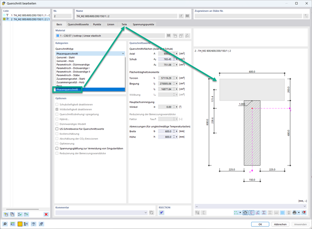
W rozszerzeniu Analiza etapów budowy (CSA) można używać przekrojów złożonych, dzięki zastosowaniu przekrojów etapowanych. Ten typ przekroju umożliwia aktywację lub dezaktywację poszczególnych części przekroju typu "Parametryczny - Masywny II" na poszczególnych etapach budowy.
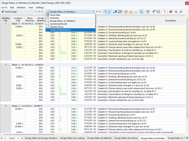
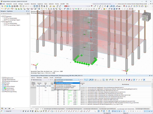
Wynik obliczeń sejsmicznych jest podzielony na dwie sekcje: wymagania dotyczące prętów i połączeń.
"Wymagania sejsmiczne" zawierają Wymaganą wytrzymałość na zginanie i Wymaganą wytrzymałość na ścinanie połączenia belka-słup dla ram sprężystych. Są one wyszczególnione w zakładce 'Połączenia ram momentowych według prętów'. W przypadku ram stężonych w zakładce 'Połączenie stężone według pręta' podawana jest Wymagana wytrzymałość połączenia na rozciąganie oraz Wymagana wytrzymałość połączenia na ściskanie stężeń.
Przeprowadzone kontrole obliczeń są przedstawiane w tabelach. W szczegółach kontroli obliczeń w przejrzysty sposób przedstawione są wzory i odniesienia do normy.
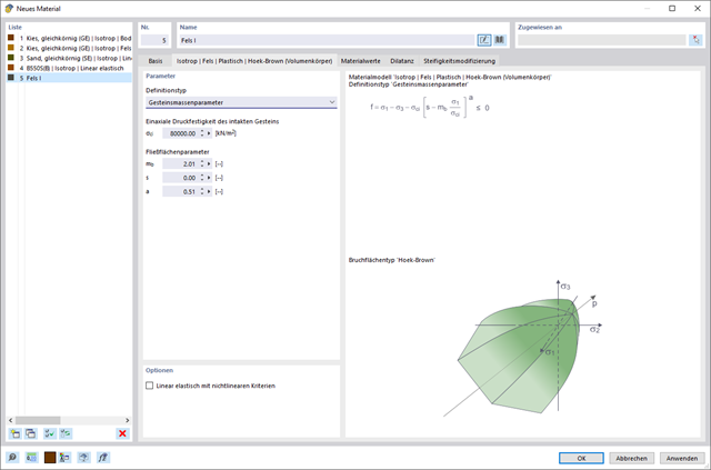
W rozszerzeniu Analiza geotechniczna dostępny jest model Hoek'a-Brown'a. Model wykazuje zachowanie materiału liniowo-sprężystego idealnie plastycznego. Jego nieliniowe kryterium wytrzymałości jest najczęściej stosowanym kryterium zniszczenia skał.
Parametry materiału można wprowadzić bezpośrednio za pomocą
- parametrów skały lub alternatywnie poprzez
- klasyfikację GSI.
opisane.
Weiterführende Informationen zu diesem Materialmodell und der Definition der Eingabe in RFEM finden Sie im entsprechenden Kapitel im Online-Handbuch für das Add-On Geotechnische Analyse: Model Hoeka-Browna .
Model budynku jest obliczany w dwóch etapach:
- Globale 3D-Berechnung des Gesamtmodells, in welchem die Decken als starre Ebene (Diaphragma) oder als Biegeplatte modelliert werden
- Lokale 2D-Berechnung der einzelnen Geschossdecken
Die Ergebnisse der Stützen und Wände aus der 3D-Berechnung und die Ergebnisse der Decken aus der 2D-Berechnung werden nach der Berechnung in einem einzigen Modell zusammengefasst. Dadurch muss zwischen dem 3D-Modell und der einzelnen 2D-Modellen der Decken nicht gewechselt werden. Der Anwender arbeitet nur mit einem Model, spart wertvolle Zeit und vermeidet eventuelle Fehler beim händischen Datenaustausch zwischen dem 3D-Modell und der einzelnen 2D-Decken-Modelle.
Die vertikalen Flächen im Modell können vom Nutzer in Schubwände (Shear Walls) und Öffnungsstürze (Sprandels) geteilt werden. Aus diesen Wandobjekten erzeugt das Programm automatisch interne Ergebnisstäbe, so dass diese dann nach der gewünschten Norm im Add-On Betonbemessung für RFEM 6 als Stäbe bemessen werden können.
Ściany usztywniające i belki-ściany z modelu budynku są dostępne jako niezależne obiekty w rozszerzeniach. W ten sposób możliwe jest szybsze filtrowanie obiektów w wynikach oraz tworzenie lepszej dokumentacji w raporcie.
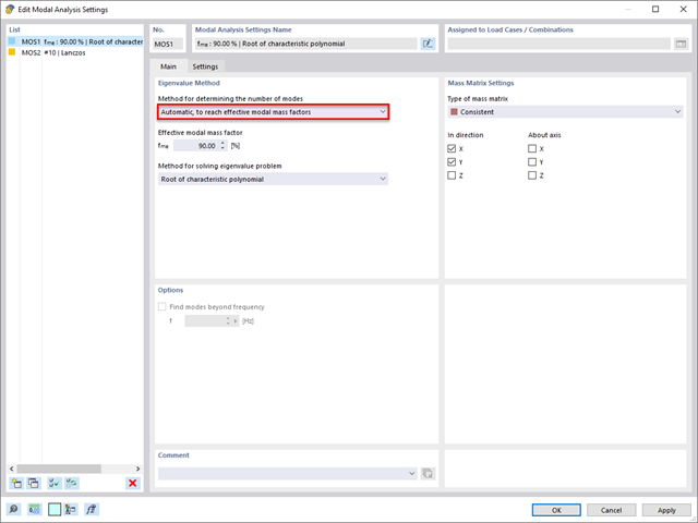
Rozszerzenie Analiza modalna umożliwia automatyczne zwiększanie poszukiwanych wartości własnych do momentu osiągnięcia zdefiniowanego współczynnika efektywnej masy modalnej. Uwzględniane są wszystkie kierunki translacyjne, które zostały aktywowane jako masy do analizy modalnej.
W ten sposób można łatwo obliczyć wymagane 90% efektywnej masy modalnej dla metody spektrum odpowiedzi.
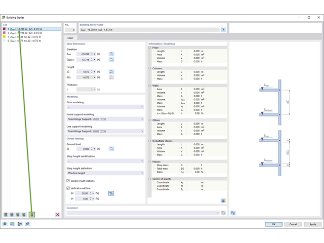
Za pomocą generatora kondygnacji w rozszerzeniu Model budynku można automatycznie tworzyć kondygnacje budynku w zależności od topologii modelu.
- 002733
- Ogólne informacje
- Projektowanie konstrukcji stalowych RFEM 6
- Projektowanie konstrukcji stalowych RSTAB 9
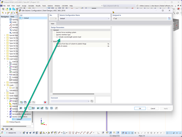
Rozszerzenie Projektowanie konstrukcji stalowych umożliwia przeprowadzanie obliczeń sejsmicznych prętów stalowych zgodnie z AISC 341-16.
W tym celu dostępnych jest pięć typów systemów SFRS (Seismic Force-Resisting Systems).

W przypadku analizy spektrum odpowiedzi modeli budynków można wyświetlić współczynniki wrażliwości dla kierunków poziomych według kondygnacji.
Dzięki tym kluczowym wartościom można zinterpretować wrażliwość na efekty stateczności.
- 002720
- Ogólne informacje
- Analiza stateczności konstrukcji RFEM 6
- Analiza stateczności konstrukcji RSTAB 9
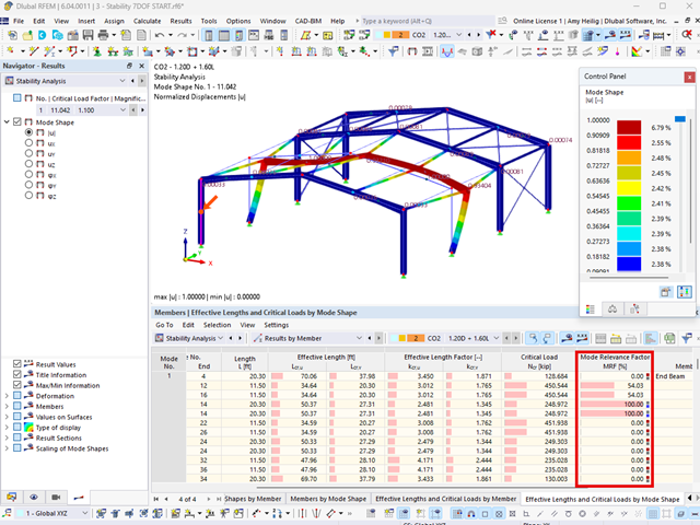
Stosując modalny współczynnik istotności (MRF) można ocenić, w jakim stopniu poszczególne elementy konstrukcyjne przyczyniają się do powstania rzeczywistego kształtu wyboczenia. Obliczenia opierają się na energii względnego odkształcenia sprężystego każdego pojedynczego pręta.
Dzięki MRF można rozróżnić lokalne i globalne kształty wyboczenia. Jeżeli kilka prętów ma znaczny MRF (np. > 20%), bardzo prawdopodobna jest niestateczność całej konstrukcji lub jej części. Jeżeli jednak suma wszystkich MRF dla kształtu drgań wynosi około 100%, należy spodziewać się lokalnego problemu ze statecznością (np. wyboczenia pojedynczego pręta).
Ponadto MRF może być wykorzystany do określenia obciążeń krytycznych i równoważnych długości wyboczeniowych poszczególnych prętów (np. do analizy stateczności). Kształty wyboczenia, dla których dany pręt ma małe wartości MRF (np. <20%), mogą zostać w tym kontekście pominięte.
MRF jest wyświetlany według kształtów wyboczenia w tabeli wyników w sekcji Analiza stateczności --> Wyniki według prętów --> Długości efektywne i obciążenia krytyczne.
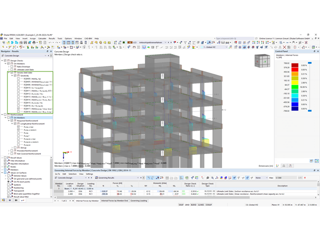
W rozszerzeniu Projektowanie konstrukcji betonowych można przeprowadzać obliczenia sejsmiczne dla prętów żelbetowych zgodnie z EC 8. Są to między innymi następujące funkcje:
- Konfiguracje obliczeń sejsmicznych
- Rozróżnianie klas ciągliwości DCL, DCM, DCH
- Możliwość przeniesienia współczynnika odpowiedzi z analizy dynamicznej
- Sprawdzenie wartości granicznej współczynnika odpowiedzi
- Weryfikacja nośności dla "Wytrzymały słup - słaba belka"
- Uszczegółowienie i reguły szczególne dla współczynnika ciągliwości krzywizny
- Uszczegółowienie i reguły szczególne dla ciągliwości lokalnej
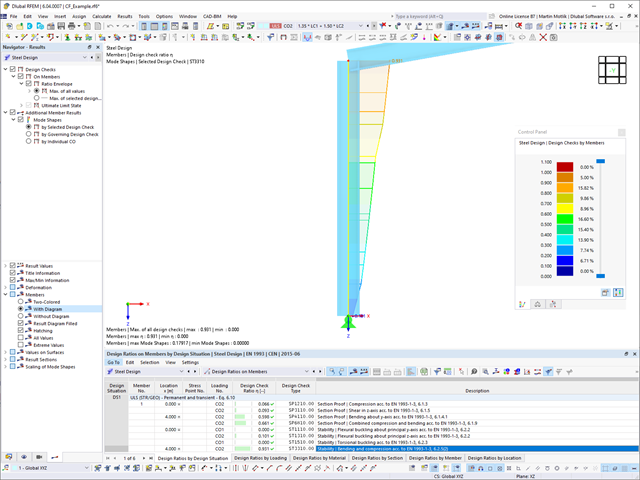
W rozszerzeniu Projektowanie konstrukcji stalowych można przeprowadzić kontrolę obliczeń stateczności i przekrojów profili formowanych na zimno według EN 1993-1-3, zgodnie z punktami 6.1.2 - 6.1.5 i 6.1.8 - 6.1.10.
Przejdź do filmu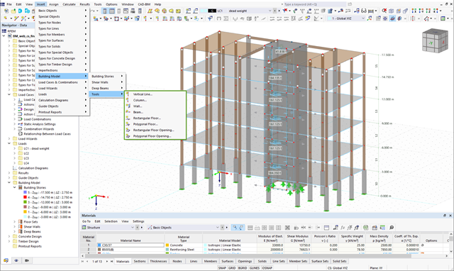
W przypadku elementów w modelach budynków dostępnych jest kilka narzędzi do modelowania:
- Linia pionowa
- Słup
- Ściana
- Belka
- Strop prostokątny
- Płyta wielokątna
- Prostokątny otwór w stropie
- Wielokątny otwór w stropie
Ta funkcja umożliwia definicję elementów na płaszczyźnie podłoża (na przykład z warstwą tła) z powiązanym tworzeniem wielu elementów w przestrzeni.
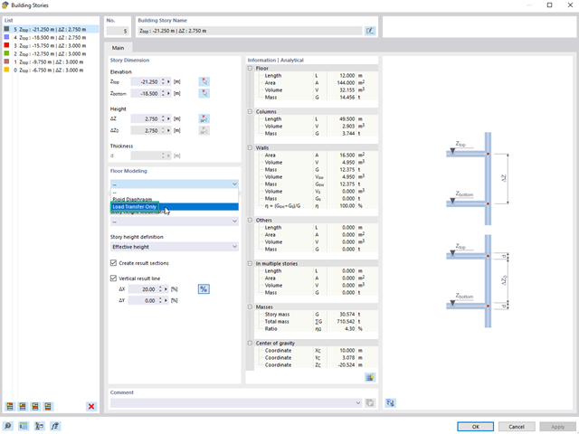
Korzystając z kondygnacji typu "Tylko przenoszenie obciążenia", można uwzględnić w rozszerzeniu Model budynku stropy bez wpływu sztywności do i z płaszczyzny. Ten typ elementu zbiera obciążenia na stropie i przenosi je na elementy nośne modelu 3D. Daje to możliwość symulacji w modelu 3D elementów drugorzędnych, takich jak np. ruszt i inne podobne elementy rozkładu obciążenia, bez dalszych efektów.
Wymiarowanie prętów stalowych formowanych na zimno zgodnie z AISI S100-16/CSA S136-16 jest dostępne w RFEM 6. Dostęp do obliczeń można uzyskać, wybierając normy „AISC 360” lub „CSA S16” w rozszerzeniu Projektowanie konstrukcji stalowych. Następnie dla obliczeń elementów formowanych na zimno automatycznie wybierane jest „AISI S100” lub „CSA S136”.
Do obliczania sprężystego obciążenia wyboczeniowego pręta program RFEM stosuje metodę DSM. Bezpośrednia metoda wytrzymałości oferuje dwa typy rozwiązań, numeryczne (metoda pasm skończonych) i analityczne (specyfikacja). Krzywą charakterystyczną (sygnaturę) FSM i kształty wyboczenia można wyświetlić w oknie dialogowym Przekroje.
- 002567
- Ogólne informacje
- Projektowanie konstrukcji stalowych RFEM 6
- Projektowanie konstrukcji stalowych RSTAB 9
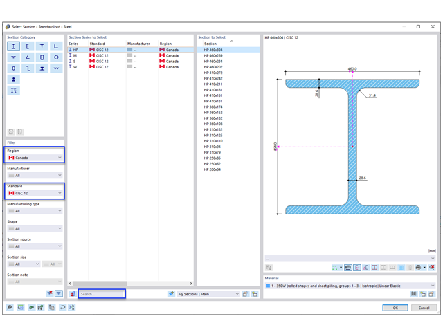
Nowe przekroje stalowe zgodnie z najnowszą instrukcją CISC (12 wydanie) są dostępne w programie RFEM 6. Przekroje są wymienione w bibliotece Znormalizowane. W filtrze należy wybrać region „Kanada”, a normę „CISC 12”. Alternatywnie nazwę przekroju można wprowadzić bezpośrednio w polu wyszukiwania znajdującym się w dolnej części okna dialogowego.
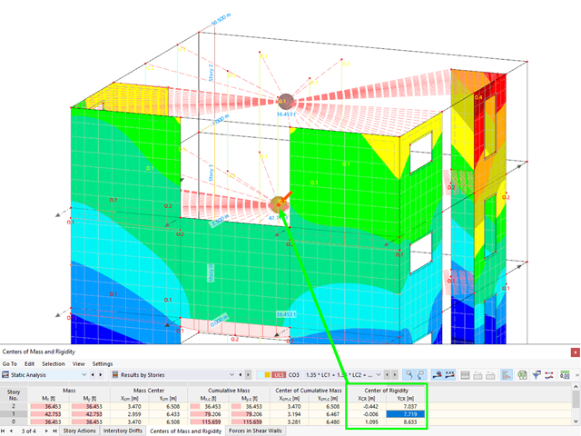
Aktywowałeś rozszerzenie Model budynku ? Bardzo dobrze! Możesz wyświetlić środek sztywności w tabeli i w formie graficznej. Użyj go na przykład do analizy dynamicznej.
.png?mw=640&hash=55038d2a1591f62179796666cb9b2fede0274e19)
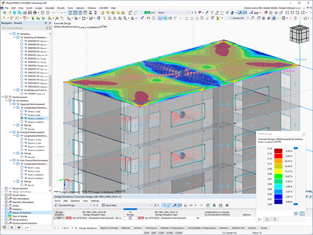
Graficzne i tabelaryczne wyświetlanie wyników dla deformacji, naprężeń i odkształceń pomaga określić bryłę gruntu. Aby to osiągnąć, skorzystaj ze specjalnych kryteriów filtrowania, które umożliwiają wybór określonych wyników.
Program na pewno cię nie zawiedzie. Jeśli chcesz graficznie ocenić wyniki w bryłach gruntu, dostępne są obiekty pomocnicze. Na przykład można zdefiniować płaszczyzny przycinania. Umożliwia to przeglądanie odpowiednich wyników na dowolnej płaszczyźnie bryły gruntu.
I nie tylko to. Wykorzystanie przekrojów wyników i brył przycinania ułatwia graficzną analizę brył gruntu.
Wiesz już, że grunt i konstrukcję można modelować i analizować w całym modelu. Oznacza to, że wyraźnie uwzględniono interakcję gleba-konstrukcja. Dostosowanie jednego elementu konstrukcyjnego prowadzi do natychmiastowego prawidłowego uwzględnienia w analizie i wynikach dla całego układu gruntu i konstrukcji.
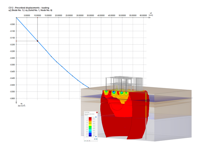
Czy jesteś gotowy na ocenę? Skorzystaj z wykresów obliczeniowych, które pokazują rozkład określonego wyniku podczas obliczeń.
Przypisanie osi pionowej i poziomej wykresu obliczeniowego można dowolnie definiować. Umożliwia to np. wyświetlenie przebiegu osiadania określonego węzła w zależności od obciążenia.
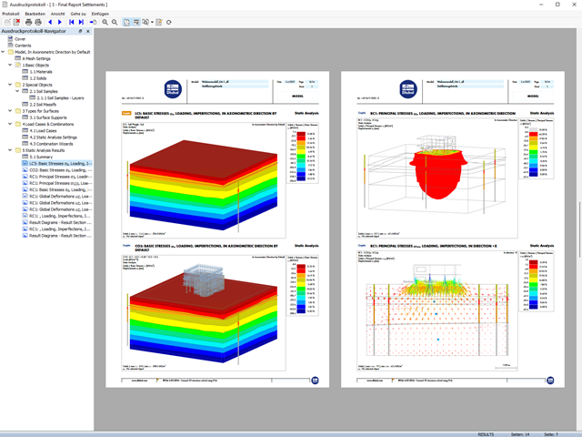
Twoje dane są zawsze dokumentowane w wielojęzycznym raporcie. W każdej chwili możesz dostosować treść i zapisać ją jako szablon. W raporcie można również za pomocą kilku kliknięć umieścić grafiki, teksty, wzory MathML i dokumenty PDF.
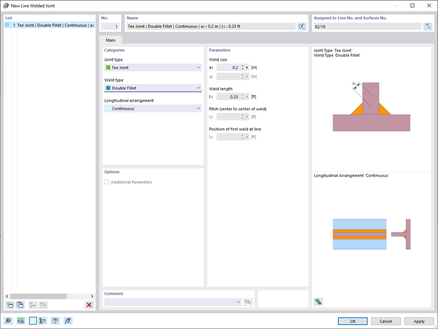
W programie RFEM 6 możliwe jest definiowanie spoin liniowych między powierzchniami i obliczanie naprężeń w spoinie za pomocą rozszerzenia Analiza naprężeniowo-odkształceniowa.
Dostępne są następujące typy połączeń:
- połączenie stykowe
- Złącze narożne
- Złącze zakładkowe
- Złącze teowe
W zależności od typu połączenia dostępne są następujące typy spoin:
- Pojedynczy kwadrat
- Podwójny
- Podwójny ukos
- Spoina typu V
- Spoina typu 2 V
- Spoina typu U
- Spoina typu 2 U
- Spoina typu J
- Spoina typu 2 J