79 Wyniki
Wyświetl wyniki:
Sortuj według:

- 002876
- Ogólne informacje
- Projektowanie konstrukcji betonowych RFEM 6
- Projektowanie konstrukcji betonowych RSTAB 9
W przypadku obliczeń betonu wyniki zbrojenia można wyświetlić w tabelach osobno w zależności od sytuacji obliczeniowych.

W rozszerzeniu Analiza geotechniczna dostępny jest pręt typu 'Pal'. Dla pala tworzone są typy nośności pala. Definiuje on parametry nośności wynikającej z tarcia na powierzchni czołowej pala oraz nośności od ciśnienia na końcu pala.
Pal jest następnie osadzany w sąsiedniej bryle gruntu z uwzględnieniem charakterystyk wytrzymałościowych wynikających z parametrów tarcia napowierzchniowego i ciśnienia szczytowego.

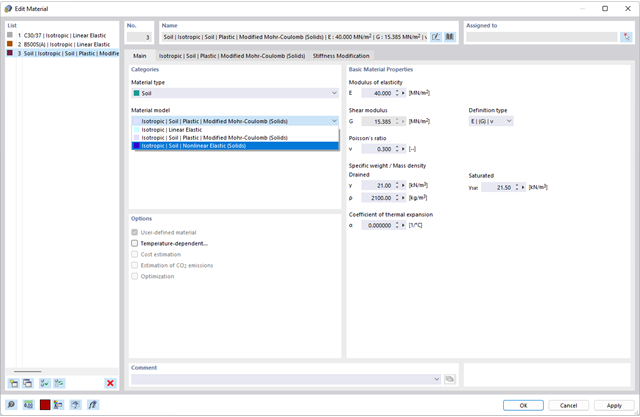
W rozszerzeniu Analiza geotechniczna dostępny jest wysokiej jakości model materiałowy "Zmodyfikowany model gruntu twardniejącego". Ten model materiałowy jest odpowiedni dla różnych gruntów i jest w stanie odpowiednio odwzorować następujące właściwości rzeczywistego gruntu.
- Zależność naprężenia od sztywności gruntu
- Zależność ścieżki obciążenia od sztywności gruntu
- Odkształcenia plastyczne jeszcze przed osiągnięciem warunku granicznego
- Wzrost wytrzymałości na ścinanie wraz ze wzrostem zagęszczenia siatki
- Wzrost granicy plastyczności wraz ze wzrostem naprężenia, aż do osiągnięcia granicznego warunku plastyczności
- Kryterium uszkodzenia według Mohra-Coulomba
Więcej informacji na temat tego modelu materiałowego oraz definicji danych wejściowych w programie RFEM można znaleźć w odpowiednim rozdziale instrukcji online rozszerzenia Analiza geotechniczna.

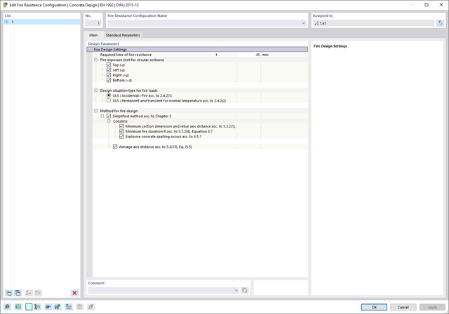
W rozszerzeniu Projektowanie konstrukcji betonowych dla programu RFEM 6 można przeprowadzić obliczenia odporności ogniowej ścian i płyt żelbetowych zgodnie z uproszczoną metodą tabelaryczną (EN 1992-1-2, rozdział 5.4.2 oraz tabele 5.8 i 5.9).

W rozszerzeniu Projektowanie konstrukcji betonowych można zdefiniować istniejące pionowe zbrojenie na ścinanie. Jest to następnie uwzględniane przy obliczaniu wytrzymałości na przebicie.
- 002801
- Ogólne informacje
- Projektowanie konstrukcji betonowych RFEM 6
- Projektowanie konstrukcji betonowych RSTAB 9
Masz indywidualne przekroje słupów i ścian o różnej geometrii, które wymagają obliczenia nośności na przebicie?
Nie ma problemu. W programie RFEM 6 można przeprowadzić obliczenia na przebicie nie tylko dla przekrojów prostokątnych i okrągłych, ale także dla dowolnego kształtu przekroju.
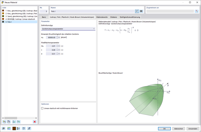
W rozszerzeniu Analiza geotechniczna dostępny jest model Hoek'a-Brown'a. Model wykazuje zachowanie materiału liniowo-sprężystego idealnie plastycznego. Jego nieliniowe kryterium wytrzymałości jest najczęściej stosowanym kryterium zniszczenia skał.
Parametry materiału można wprowadzić bezpośrednio za pomocą
- parametrów skały lub alternatywnie poprzez
- klasyfikację GSI.
opisane.
Weiterführende Informationen zu diesem Materialmodell und der Definition der Eingabe in RFEM finden Sie im entsprechenden Kapitel im Online-Handbuch für das Add-On Geotechnische Analyse: Model Hoeka-Browna .
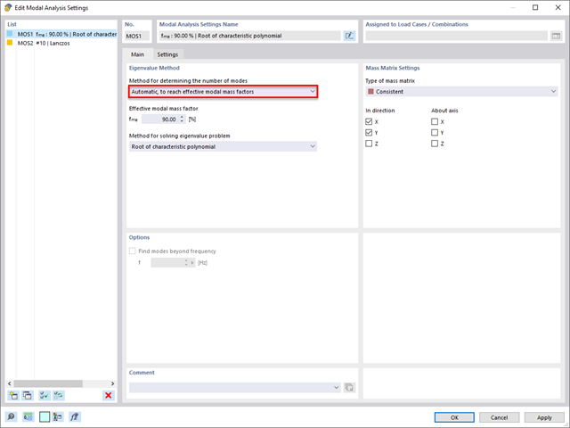
Rozszerzenie Analiza modalna umożliwia automatyczne zwiększanie poszukiwanych wartości własnych do momentu osiągnięcia zdefiniowanego współczynnika efektywnej masy modalnej. Uwzględniane są wszystkie kierunki translacyjne, które zostały aktywowane jako masy do analizy modalnej.
W ten sposób można łatwo obliczyć wymagane 90% efektywnej masy modalnej dla metody spektrum odpowiedzi.

W przypadku analizy spektrum odpowiedzi modeli budynków można wyświetlić współczynniki wrażliwości dla kierunków poziomych według kondygnacji.
Dzięki tym kluczowym wartościom można zinterpretować wrażliwość na efekty stateczności.
- 002720
- Ogólne informacje
- Analiza stateczności konstrukcji RFEM 6
- Analiza stateczności konstrukcji RSTAB 9
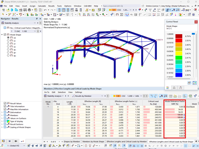
Stosując modalny współczynnik istotności (MRF) można ocenić, w jakim stopniu poszczególne elementy konstrukcyjne przyczyniają się do powstania rzeczywistego kształtu wyboczenia. Obliczenia opierają się na energii względnego odkształcenia sprężystego każdego pojedynczego pręta.
Dzięki MRF można rozróżnić lokalne i globalne kształty wyboczenia. Jeżeli kilka prętów ma znaczny MRF (np. > 20%), bardzo prawdopodobna jest niestateczność całej konstrukcji lub jej części. Jeżeli jednak suma wszystkich MRF dla kształtu drgań wynosi około 100%, należy spodziewać się lokalnego problemu ze statecznością (np. wyboczenia pojedynczego pręta).
Ponadto MRF może być wykorzystany do określenia obciążeń krytycznych i równoważnych długości wyboczeniowych poszczególnych prętów (np. do analizy stateczności). Kształty wyboczenia, dla których dany pręt ma małe wartości MRF (np. <20%), mogą zostać w tym kontekście pominięte.
MRF jest wyświetlany według kształtów wyboczenia w tabeli wyników w sekcji Analiza stateczności --> Wyniki według prętów --> Długości efektywne i obciążenia krytyczne.
- 002691
- Ogólne informacje
- Projektowanie konstrukcji betonowych RFEM 6
- Projektowanie konstrukcji betonowych RSTAB 9
W rozszerzeniu Projektowanie konstrukcji betonowych można przeprowadzić uproszczone obliczenia odporności ogniowej słupów (Rozdział 5.3.2) i belek (Rozdział 5.6), zgodnie z EN 1992-1-2.
W przypadku uproszczonych obliczeń odporności ogniowej dostępne są następujące metody weryfikacji:
- Słupy: Minimalne wymiary przekroju prostokątnego i okrągłego wg tabeli 5.2a oraz równania 5.7 do obliczania czasu ekspozycji pożarowej
- Belki: Minimalne wymiary i odległości między środkami zgodnie z Tabelą 5.5 i Tabelą 5.6
Siły wewnętrzne do obliczeń odporności ogniowej można wyznaczyć przy użyciu dwóch metod.
- 1: W tym przypadku siły wewnętrzne z wyjątkowej sytuacji obliczeniowej są bezpośrednio uwzględniane w obliczeniach.
- 2: Siły wewnętrzne z obliczeń w temperaturze normalnej są redukowane za pomocą współczynnika Eta,fi (ηfi) i są następnie wykorzystywane do obliczeń odporności ogniowej.
Ponadto istnieje możliwość modyfikacji rozstawu osi zgodnie z równ. 5.5.
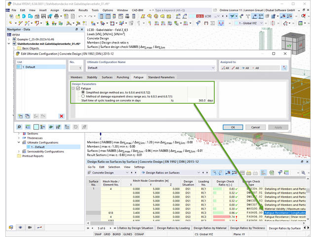
Rozszerzenie Projektowanie konstrukcji betonowych umożliwia wymiarowanie prętów i powierzchni ze względu na zmęczenie zgodnie z EN 1992-1-1, rozdział 6.8.
W przypadku obliczeń zmęczenia można opcjonalnie wybrać dwie metody lub poziomy obliczeniowe w konfiguracjach obliczeniowych:
- Poziom obliczeniowy 1: Obliczenia uproszczone wg. do 6.8.6 i 6.8.7(2) Kryterium uproszczone jest stosowane dla częstych kombinacji oddziaływań zgodnie z EN 1992-1-1, rozdział 6.8.6 (2) oraz EN 1990, równ. (6.15b) wraz z obciążeniami od ruchu drogowego w stanie użytkowalności. Dla stali zbrojeniowej sprawdzany jest maksymalny zakres naprężeń zgodnie z 6.8.6. Naprężenie ściskające w betonie jest określane za pomocą górnego i dolnego dopuszczalnego naprężenia zgodnie z 6.8.7(2).
- Poziom analizy 2: Obliczanie równoważnego naprężenia niszczącego zgodnie z 6.8.5 i 6.8.7(1) (uproszczone obliczenia na zmęczenie): Obliczenia z wykorzystaniem zakresów równoważnych naprężeń niszczących są przeprowadzane dla kombinacji zmęczeniowych, zgodnie z EN 1992-1-1, rozdział 6.8.3, równ. (6.69) o specyficznie zdefiniowanym oddziaływaniu cyklicznym Qfat .
W rozszerzeniu Projektowanie konstrukcji betonowych można przeprowadzać obliczenia sejsmiczne dla prętów żelbetowych zgodnie z EC 8. Są to między innymi następujące funkcje:
- Konfiguracje obliczeń sejsmicznych
- Rozróżnianie klas ciągliwości DCL, DCM, DCH
- Możliwość przeniesienia współczynnika odpowiedzi z analizy dynamicznej
- Sprawdzenie wartości granicznej współczynnika odpowiedzi
- Weryfikacja nośności dla "Wytrzymały słup - słaba belka"
- Uszczegółowienie i reguły szczególne dla współczynnika ciągliwości krzywizny
- Uszczegółowienie i reguły szczególne dla ciągliwości lokalnej
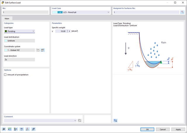
Wprowadzenie typu obciążenia Woda stojąca umożliwia symulację oddziaływań deszczu na powierzchnie wielokrotnie zakrzywione, z uwzględnieniem przemieszczeń według analizy dużych odkształceń.
Ten numeryczny proces analizy deszczowej analizuje przypisaną geometrię powierzchni i określa, które składowe wody deszczowej spływają, a które gromadzą się w postaci kałuży (kieszeni wodnych) na powierzchni. Rozmiar kałuży powoduje wówczas odpowiednie obciążenie pionowe do analizy statyczno-wytrzymałościowej.
Funkcja ta jest przeznaczona do analizy w przybliżeniu poziomych geometrii dachów membranowych pod obciążeniem deszczem.
Przejdź do filmu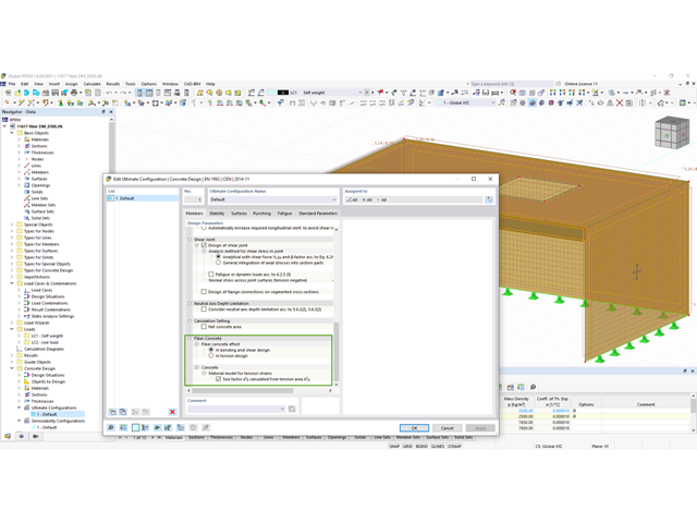
Teraz w rozszerzeniu Projektowanie konstrukcji betonowych można wymiarować elementy wykonane z betonu zbrojonego włóknami zgodnie z wytyczną "DAfStb Steel Fiber-Reinforced Concrete".
Ta opcja jest dostępna dla obliczeń zgodnie z EN 1992-1-1. Obliczenia zgodnie z wytyczną DAfStb są przeprowadzane po przypisaniu betonu typu "Fibrobeton" do elementu konstrukcyjnego z betonu zbrojonego.
Przejdź do filmu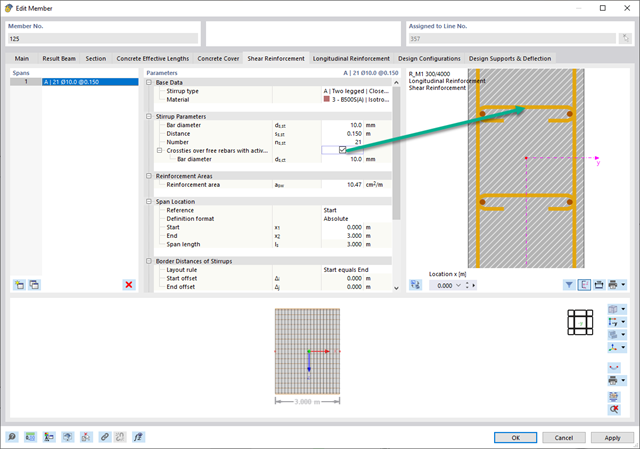
W zakładce "Zbrojenie na ścinanie" można wybrać opcję "Powiązania krzyżowe na wolnych prętach zbrojeniowych z aktywnym wyborem w oknie graficznym". Pozwala to na umieszczenie dodatkowych powiązań krzyżowych na wolnych prętach zbrojenia podłużnego.
Pozycję więzów krzyżowych można aktywować lub dezaktywować w infografice. Powiązania krzyżowe są uwzględniane podczas kontroli stanu granicznego nośności i obliczeń konstrukcji. Są one dostępne dla obliczeń zgodnie z EN 1992-1-1.
Przejdź do filmu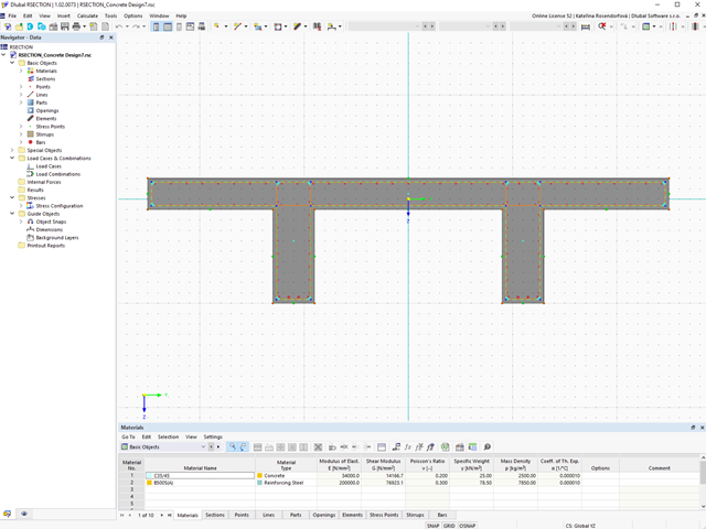
W rozszerzeniu Projektowanie konstrukcji betonowych można wymiarować dowolny przekrój RSECTION. Otulinę betonową, zbrojenie na ścinanie i zbrojenie podłużne definiuje się bezpośrednio w RSECTION.
Po zaimportowaniu przekroju ze zbrojeniem RSECTION do programu RFEM 6, można go również wykorzystać do obliczeń w rozszerzeniu Projektowanie konstrukcji betonowych.
Przejdź do filmu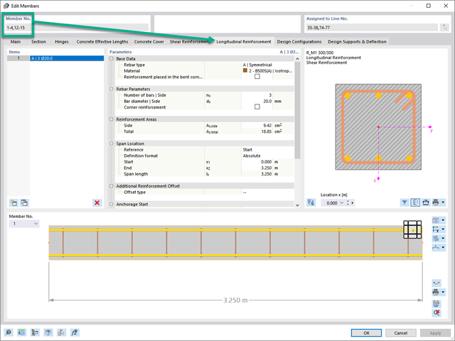
- 002557
- Ogólne informacje
- Projektowanie konstrukcji betonowych RFEM 6
- Projektowanie konstrukcji betonowych RSTAB 9
Skorzystaj i oszczędzaj czas! Ta funkcja umożliwia jednoczesne definiowanie lub edycję zbrojenia dla kilku prętów lub zbiorów prętów.
Przejdź do filmu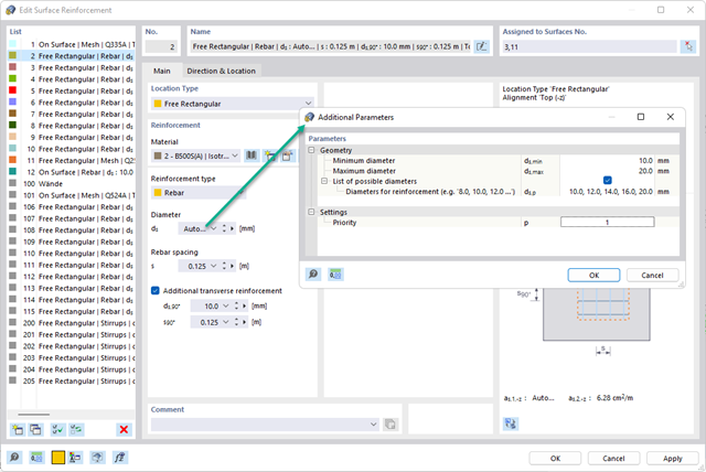
Istniejące zbrojenie powierzchniowe można automatycznie zaprojektować tak, aby pokryć wymagane zbrojenie. Można wybrać, czy automatycznie ma być definiowana średnica zbrojenia, czy też rozstaw prętów.
Przejdź do filmu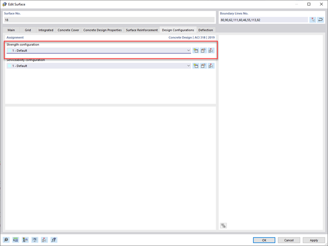
- 002469
- Ogólne informacje
- Projektowanie konstrukcji betonowych RFEM 6
- Projektowanie konstrukcji betonowych RSTAB 9
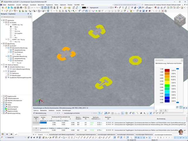
Pracujesz z elementami konstrukcyjnymi składającymi się z płyt? W takim przypadku należy przeprowadzić obliczenia na ścinanie z uwzględnieniem wymagań obliczania przebicia, na przykład zgodnie z 6.4, EN 1992-1-1. Oprócz płyt stropowych można w ten sposób wymiarować również płyty fundamentowe.
W konfiguracji stanu granicznego nośności dla wymiarowania betonu można zdefiniować parametry obliczeń przebicia dla wybranych węzłów.
.png?mw=640&hash=55038d2a1591f62179796666cb9b2fede0274e19)
Graficzne i tabelaryczne wyświetlanie wyników dla deformacji, naprężeń i odkształceń pomaga określić bryłę gruntu. Aby to osiągnąć, skorzystaj ze specjalnych kryteriów filtrowania, które umożliwiają wybór określonych wyników.
Program na pewno cię nie zawiedzie. Jeśli chcesz graficznie ocenić wyniki w bryłach gruntu, dostępne są obiekty pomocnicze. Na przykład można zdefiniować płaszczyzny przycinania. Umożliwia to przeglądanie odpowiednich wyników na dowolnej płaszczyźnie bryły gruntu.
I nie tylko to. Wykorzystanie przekrojów wyników i brył przycinania ułatwia graficzną analizę brył gruntu.
Wiesz już, że grunt i konstrukcję można modelować i analizować w całym modelu. Oznacza to, że wyraźnie uwzględniono interakcję gleba-konstrukcja. Dostosowanie jednego elementu konstrukcyjnego prowadzi do natychmiastowego prawidłowego uwzględnienia w analizie i wynikach dla całego układu gruntu i konstrukcji.
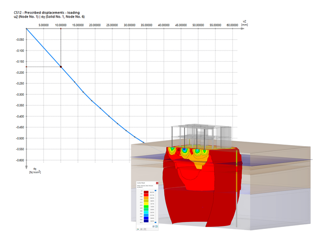
Czy jesteś gotowy na ocenę? Skorzystaj z wykresów obliczeniowych, które pokazują rozkład określonego wyniku podczas obliczeń.
Przypisanie osi pionowej i poziomej wykresu obliczeniowego można dowolnie definiować. Umożliwia to np. wyświetlenie przebiegu osiadania określonego węzła w zależności od obciążenia.
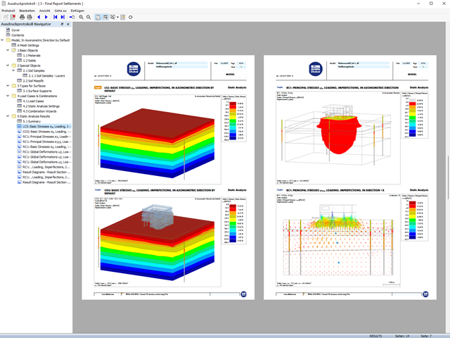
Twoje dane są zawsze dokumentowane w wielojęzycznym raporcie. W każdej chwili możesz dostosować treść i zapisać ją jako szablon. W raporcie można również za pomocą kilku kliknięć umieścić grafiki, teksty, wzory MathML i dokumenty PDF.
Wprowadzenie i modelowanie bryły gruntowej bezpośrednio w programie RFEM. Modele materiałów gruntowych można łączyć ze wszystkimi popularnymi rozszerzeniami dla programu RFEM.
Umożliwia to łatwą analizę całych modeli z pełną prezentacją interakcji grunt-konstrukcja.
Wszystkie parametry wymagane do obliczeń są określane automatycznie na podstawie wprowadzonych danych materiałowych. Następnie program generuje krzywe naprężenie-odkształcenie dla każdego elementu ES.
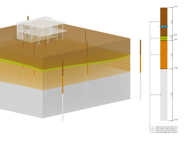
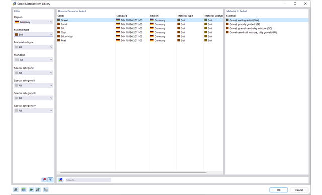
Czy wiecie, że...? Uwarstwienie gruntu, pobrane z raportów o podłożu gruntowym w miejscach wychodni, można wprowadzić bezpośrednio do programu w postaci próbek gruntu. Przypisz badane materiały gruntowe wraz z ich właściwościami do warstw.
Za pomocą danych tabelarycznych i okna dialogowego edycji można zdefiniować próbkę. Można również określić poziom wód gruntowych w próbkach gruntu.
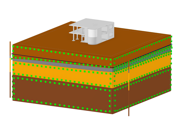
Bryły gruntu, które mają zostać przeanalizowane, są sumowane w masywach gruntu.
Próbki gruntu należy wykorzystać jako podstawę do zdefiniowania masywu gruntowego. W ten sposób program umożliwia generowanie masywu w sposób przyjazny dla użytkownika, w tym automatyczne określanie granic faz na podstawie danych z próbki, a także poziomu wód gruntowych i podpór powierzchni granicznej.
Masywy gruntowe umożliwiają określenie docelowego rozmiaru siatki ES niezależnie od ustawień globalnych dla reszty konstrukcji. Dzięki temu w całym modelu można uwzględnić różne wymagania dotyczące budynku i gruntu.
Czy chcesz modelować i analizować zachowanie bryły gruntowej? Aby to zapewnić, w programie RFEM zaimplementowano odpowiednie modele materiałowe.
Można użyć zmodyfikowanego modelu Mohra-Coulomba z liniowo-sprężystym modelem idealnie plastycznym lub nieliniowo sprężystym modelem z edometryczną relacją naprężenie-odkształcenie. Kryterium graniczne, które opisuje przejście od obszaru sprężystości do obszaru płynięcia plastycznego, jest zdefiniowane według Mohra-Coulomba.
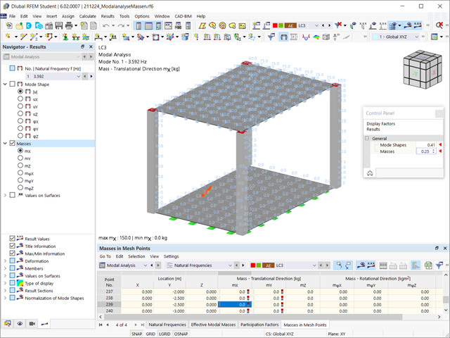
Czy odkryłeś już tabelaryczne i graficzne przedstawianie mas w punktach siatki? Po prawej, jest to również jeden z wyników analizy modalnej w programie RFEM 6. W ten sposób można sprawdzić importowane masy, które zależą od różnych ustawień analizy modalnej. Mogą być one wyświetlane w zakładce Masy w punktach siatki tabeli Wyniki. Tabela zawiera przegląd następujących wyników: Masa - kierunek przesuwny (mX, mY, mZ ), Masa - kierunek obrotowy (mφX, mφY, mφZ ) oraz suma mas. Czy nie byłoby lepiej, gdybyś jak najszybciej przeprowadził ocenę graficzną? Następnie można również wyświetlić graficznie masy w punktach siatki.
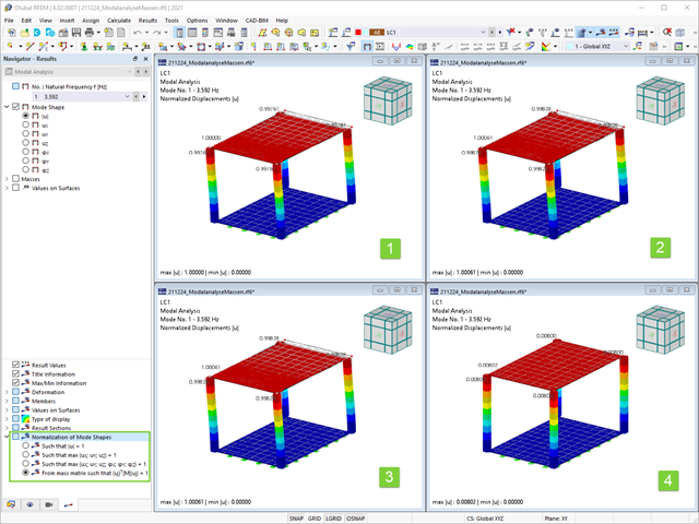
Jak już wiesz, po pomyślnym zakończeniu obliczeń wyniki przypadku obciążenia w Analizie modalnej są wyświetlane w programie. Die erste Eigenform ist für Sie also sofort grafisch oder animiert zu sehen. Dabei können Sie die Darstellung der Eigenformnormierung komfortabel anpassen. Erledigen Sie das am besten direkt im Ergebnisnavigator, wo Sie zur Visualisierung der Eigenformen eine von vier Optionen auswählen:
- Wert des Eigenformvektors uj auf 1 skalieren (berücksichtigt nur die Translationskomponenten)
- Auswahl der maximalen Translationskomponente des Eigenvektors und Einstellung auf 1
- Betrachtung der gesamten Eigenform (inklusive der Rotationskomponenten), Auswahl des Maximums und Einstellung auf 1
- Setzen der modalen Massen mi für jeden Eigenwert auf 1 kg
Ausführlichere Erläuterungen der Normierung der Eigenformen finden Sie hier: Instrukcja online .