48 Wyniki
Wyświetl wyniki:
Sortuj według:
- Proste definiowanie etapów budowy konstrukcji w RFEM wraz z wizualizacją
- Dodawanie, usuwanie, modyfikowanie i reaktywacja elementów prętowych, powierzchniowych i bryłowych oraz ich właściwości (np. przeguby prętowe i liniowe, stopnie swobody dla podpór itp.)
- Ręczna oraz automatyczna kombinatoryka obciążeń na poszczególnych etapach budowy konstrukcji (np. w celu uwzględnienia obciążeń montażowych, tymczasowych urządzeń dźwigowych itp.)
- Uwzględnienie wpływów nieliniowych, takich jak uszkodzenie prętów rozciąganych lub nieliniowe zachowanie podpór
- Interakcja z innymi rozszerzeniami, takimi jak z. B. Nieliniowe zachowanie materiału, Stateczność konstrukcji, -rstab-9/additional-analyses/form-finding/form-finding itd.
- Wyświetlanie wyników w postaci numerycznej i graficznej dla poszczególnych etapów budowy
- Szczegółowy protokół wydruku wraz z dokumentacją wszystkich danych konstrukcyjnych i obciążeń dla każdego etapu budowy
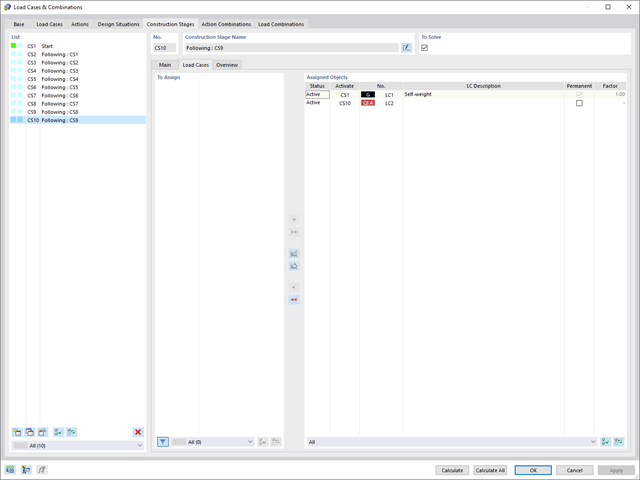
Czy udało Ci się utworzyć całą konstrukcję w programie RFEM? Dobrze, teraz można przypisać poszczególne elementy konstrukcyjne i przypadki obciążeń do odpowiednich etapów budowy. Na każdym etapie budowy można modyfikować na przykład definicje zwolnień prętów i podpór.
Pozwala to na modelowanie zmian konstrukcyjnych, na przykład podczas betonowania dźwigarów mostowych lub osiadania słupów. Przypadki obciążeń utworzone w programie RFEM należy następnie przydzielić do etapów budowy jako obciążenia stałe lub przejściowe.
Czy wiecie, że...? Kombinatoryka umożliwia nakładanie obciążeń stałych i przejściowych w kombinacjach obciążeń. W ten sposób można określić maksymalne siły wewnętrzne dla różnych pozycji dźwigu lub uwzględnić tymczasowe obciążenia montażowe dostępne tylko w jednym etapie budowy.
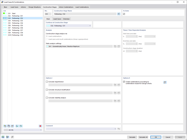
Jeżeli między idealnym układem a układem, który uległ deformacji z poprzedniego etapu budowy, pojawią się różnice w geometrii, są one porównywane w programie. Następujące po sobie kolejne etapy budowy obliczane są na bazie układu konstrukcyjnego z odkształceniami i obciążeniami wynikającymi z poprzednich etapu budowy. Obliczenia te są nieliniowe.
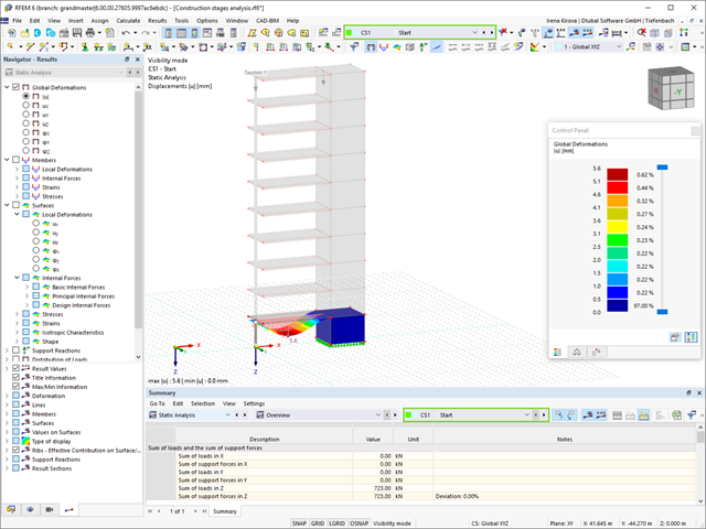
Czy obliczenia zakończyły się pomyślnie? Wyniki poszczególnych etapów budowy można teraz wyświetlać graficznie oraz w tabelach w programie RFEM. Ponadto program RFEM umożliwia uwzględnienie etapów budowy w kombinatoryce i uwzględnienie ich w dalszych obliczeniach.
_ENG.png?mw=640&hash=1053c9bef400e9f5361c9c3278f76a272fcc4ddf)
Czy aktywowałeś rozszerzenie Analiza historii czasowej (TDA)? Dobrze, teraz można dodawać dane czasowe do przypadków obciążeń. Po zdefiniowaniu początku i końca obciążenia, uwzględniany jest wpływ pełzania na końcu obciążenia. Program umożliwia modelowanie efektów pełzania w konstrukcjach szkieletowych i kratowych wykonanych z betonu zbrojonego.
W tym przypadku obliczenia są przeprowadzane nieliniowo zgodnie z modelem reologicznym (model Kelvina i Maxwella).
Czy obliczenia zakończyły się pomyślnie? Wyznaczone siły wewnętrzne można teraz wyświetlić w tabelach i grafice, a także uwzględnić w obliczeniach.
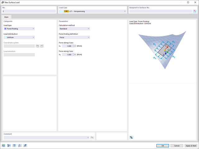
Po aktywowaniu rozszerzenia Form-Finding w Danych ogólnych, efekt znajdowania kształtu jest przypisywany do przypadków obciążeń z kategorią przypadków obciążenia "Sprężenie" w połączeniu z obciążeniami od znajdowania kształtu od pręta, powierzchni i bryły wczytaj katalog. Jest to przypadek obciążenia wstępnego naprężenia. Przekształca się on zatem w analizę znajdowania kształtu dla całego modelu ze zdefiniowanymi w nim wszystkimi elementami prętowymi, powierzchniowymi i bryłowymi. Do znajdowania kształtu odpowiednich elementów prętowych i membranowych dochodzi się w całym modelu za pomocą specjalnych obciążeń w zakresie znajdowania kształtu i regularnych definicji obciążeń. Te obciążenia znajdowania kształtu opisują oczekiwany stan odkształcenia lub siły po wyszukaniu kształtu w elementach. Obciążenia regularne opisują zewnętrzne obciążenie całego układu.
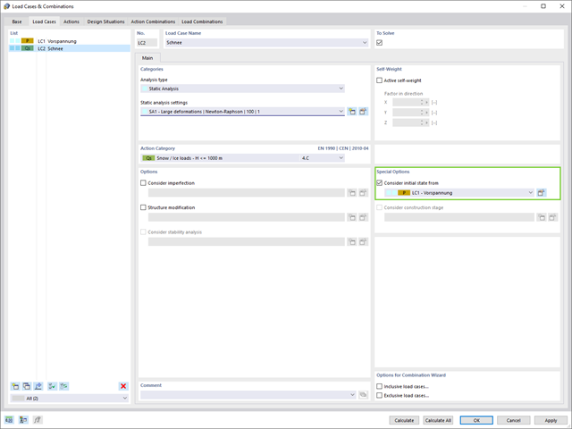
Czy wiesz dokładnie, w jaki sposób przebiega wyszukiwanie kształtu? Po pierwsze, proces znajdowania kształtu przypadków obciążeń z kategorią przypadku obciążenia "Wstępne naprężenie" przesuwa początkową geometrię siatki do optymalnie zrównoważonej pozycji za pomocą iteracyjnych pętli obliczeniowych. W tym celu program wykorzystuje metodę Zaktualizowanej Strategii Odniesienia (URS) opracowaną przez prof. Bletzingera i prof. Ramma. Technologię tę charakteryzują kształty równowagi, które po obliczeniach prawie dokładnie odpowiadają początkowo zadanym warunkom brzegowym (ugięcie, siła i naprężenie wstępne).
Oprócz opisu oczekiwanych sił lub zwisów na elementach, zintegrowane podejście URS umożliwia również uwzględnienie sił regularnych. W całym procesie pozwala to na przykład na opisanie ciężaru własnego lub ciśnienia pneumatycznego za pomocą odpowiednich obciążeń elementów.
Wszystkie te opcje dają rdzeniu obliczeniowemu możliwość obliczania postaci antyklastycznych i synklastycznych, które są w równowadze sił, dla geometrii płaskich lub obrotowo-symetrycznych. Aby możliwe było realistyczne zaimplementowanie obu typów, pojedynczo lub razem w jednym środowisku, w obliczeniach dostępne są dwa sposoby opisania wektorów sił do analizy form-finding:
- Metoda rozciągania - opis znajdowania kształtu wektorów sił w przestrzeni dla geometrii płaskich
- Metoda rzutowania - opis znajdowania kształtu wektorów sił na płaszczyznę rzutowania z ustaleniem położenia poziomego dla geometrii stożkowych
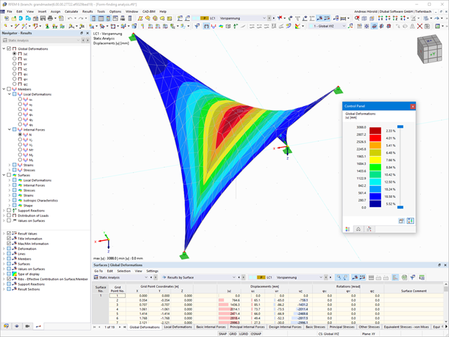
Proces znajdowania kształtu tworzy model konstrukcyjny z aktywnymi siłami w "przypadku obciążenia sprężonego" Ten przypadek obciążenia pokazuje przemieszczenie od początkowego położenia wejściowego do ustalonej geometrii w wynikach deformacji. W wynikach opartych na sile lub naprężeniach (siły wewnętrzne prętów i powierzchni, naprężenia w bryłach, ciśnienia gazu itp.) określany jest stan w celu zachowania znalezionej formy. Do analizy kształtu geometrycznego program oferuje dwuwymiarowy wykres konturowy z przedstawieniem wysokości bezwzględnej i wykresem nachylenia do wizualizacji sytuacji na zboczu.
Teraz przeprowadzane są dalsze obliczenia i analiza statyczno-wytrzymałościowa całego modelu. W tym celu program przenosi geometrię zorientowaną na kształt wraz z odkształceniami zależnymi od elementów do uniwersalnego stanu początkowego. Można go teraz używać w przypadkach obciążeń i kombinacjach obciążeń.
W porównaniu z modułem dodatkowym RF-/STAGES (RFEM 5) do rozszerzenia Analiza etapów budowy (CSA) dla programu RFEM 6 dodano następujące nowe funkcje:
- Uwzględnienie etapów budowy na poziomie programu RFEM
- Integracja analizy etapu budowy z kombinatoryką w programie RFEM
- Wprowadzono podparcie dla dodatkowych elementów konstrukcyjnych, takich jak przeguby liniowe
- Analiza alternatywnych procesów konstrukcyjnych w modelu
- Ponowna aktywacja elementów konstrukcyjnych
W porównaniu z modułem dodatkowym RF-FORM-FINDING (RFEM 5), do modułu Form-Finding dla programu RFEM 6 dodano następujące nowe funkcje:
- Określenie wszystkich warunków brzegowych dotyczących obciążenia dla analizy znajdowania kształtu (form-finding) w pojedynczym przypadku obciążenia
- Przechowywanie wyników analizy znajdowania kształtu jako stanu początkowego z możliwością późniejszego wykorzystania przy dalszej analizie modelu
- Automatyczne przypisywanie stanu początkowego z analizy znajdowania kształtu do wszystkich sytuacji obciążeniowych w sytuacji obliczeniowej za pomocą kreatorów kombinacji
- Dodatkowe geometryczne warunki brzegowe dla prętów (długość elementu nieobciążonego, maksymalny zwis w pionie, zwis w pionie w najniższym punkcie punkcie)
- Dodatkowe warunki brzegowe z uwagi na obciążenie w analizie znajdowania kształtu dla prętów (maksymalna siła w pręcie, minimalna siła w pręcie, rozciągająca składowa pozioma, rozciąganie na i-końcu, rozciąganie na końcu j, minimalne rozciąganie na końcu i, minimalne rozciąganie na końcu j)
- Typ materiału „Tkanina” i „Folia” w bibliotece materiałów
- Równoległe analizy znajdowania kształtu w jednym modelu
- Symulacja kolejnych etapów znajdowania kształtów w połączeniu z rozszerzeniem Analiza etapów konstrukcji (CSA)
- 002172
- Ogólne informacje
- Projektowanie konstrukcji drewnianych RFEM 6
- Projektowanie konstrukcji drewnianych RSTAB 9
W porównaniu z modułem dodatkowym RF-/TIMBER Pro (RFEM 5/RSTAB 8) do rozszerzenia Projektowanie konstrukcji drewnianych dla programu RFEM 6/RSTAB 9 dodano następujące nowe funkcje:
- Oprócz Eurokodu 5, uwzględnione zostały inne międzynarodowe normy (SIA 265, ANSI/AWC NDS, CSA O86, GB 50005)
- Obliczanie ściskania prostopadle do włókien (ciśnienie na podporze)
- Wprowadzenie solwera wartości własnych do wyznaczania momentu krytycznego dla wyboczenia skrętnego (tylko EC 5)
- Definicja różnych długości efektywnych do obliczeń w normalnej temperaturze i odporności ogniowej
- Ocena naprężeń poprzez naprężenia jednostkowe (MES)
- Zoptymalizowane analizy stateczności dla prętów o zbieżnym przekroju
- Ujednolicenie materiałów dla wszystkich załączników krajowych (w bibliotece materiałów dostępna jest teraz tylko jedna norma „EN”)
- Wyświetlanie osłabień przekrojów bezpośrednio w renderingu
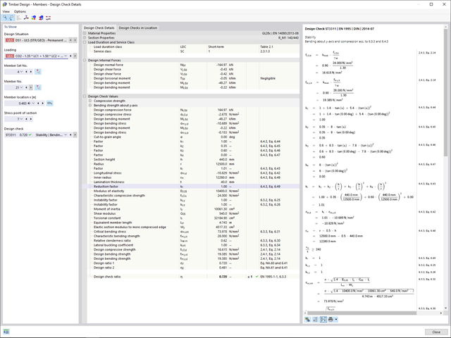
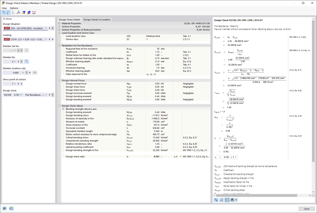
- Wyświetlanie odpowiednich wzorów użytych do sprawdzania warunków nośności (w tym odniesienie do zastosowanego równania z normy)

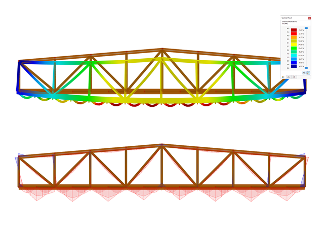
Dla każdego przypadku obciążenia można wyświetlić odkształcenia w czasie końcowym.
Wyniki te są również dokumentowane w protokole wydruku programów RFEM i RSTAB. Zawartość protokołu i jego zakres można wybrać specjalnie dla poszczególnych warunków projektowych.
Dzięki rozszerzeniu Analiza historii czasowej (TDA) można uwzględnić zmienne w czasie zachowanie materiału w przypadku prętów i powierzchni. Długotrwałe efekty, takie jak pełzanie, skurcz i starzenie, mogą wpływać na rozkład sił wewnętrznych, w zależności od konstrukcji. Darauf bereiten Sie sich mit diesem Add-On optimal vor.
- 002369
- Ogólne informacje
- Projektowanie konstrukcji drewnianych RFEM 6
- Projektowanie konstrukcji drewnianych RSTAB 9
- Obliczanie ugięć i porównanie z normatywnymi lub ręcznie dostosowanymi wartościami granicznymi
- Uwzględnienie wygięcia wstępnego w analizie ugięcia
- W zależności od typu sytuacji obliczeniowej możliwe są różne wartości graniczne
- Ręczne dostosowywanie długości odniesienia i segmentacji według kierunku
- Obliczanie ugięć w odniesieniu do konstrukcji początkowej lub do konstrukcji odkształconej
- Automatyczne uwzględnienie odkształceń zależnych od czasu poprzez zwiększenie obciążenia o współczynnik pełzania (może być również zdefiniowany przez użytkownika po stronie sztywności)
- Uproszczone obliczenia drgań
- Graficzne wyświetlanie wyników zintegrowane z RFEM/RSTAB; na przykład stopień wykorzystania wartości granicznej, odkształcenie lub ugięcie
- Pełna integracja wyników z protokołem wydruku programu RFEM/RSTAB
- 002370
- Ogólne informacje
- Projektowanie konstrukcji drewnianych RFEM 6
- Projektowanie konstrukcji drewnianych RSTAB 9
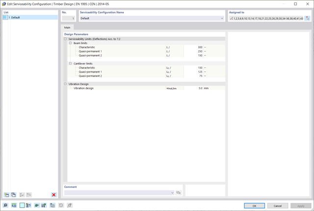
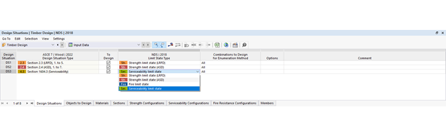
Za wygenerowanie i obliczenie kombinacji obciążeń i wyników wymaganych dla stanu granicznego użytkowalności odpowiada program RFEM/RSTAB. W rozszerzeniu Projektowanie konstrukcji drewnianych można wybrać sytuacje obliczeniowe do analizy ugięć. Obliczone wartości odkształceń są następnie określane w każdym miejscu pręta, w zależności od określonego wygięcia wstępnego i układu odniesienia, a następnie porównywane z wartościami granicznymi.
Wartość graniczną deformacji można określić indywidualnie dla każdego elementu konstrukcyjnego w Konfiguracja stanu granicznego użytkowalności. W takim przypadku maksymalne odkształcenie nie powinno przekraczać dopuszczalnej wartości granicznej, zależnej od długości odniesienia. Podczas definiowania podpór obliczeniowych można podzielić komponenty na segmenty. Umożliwia to automatyczne określenie odpowiedniej długości odniesienia dla każdego kierunku obliczeń.
Na podstawie położenia przypisanych podpór obliczeniowych program automatycznie określa różnicę między belkami a wspornikami. W ten sposób można mieć pewność, że wartość graniczna zostanie odpowiednio określona.
- 002371
- Ogólne informacje
- Projektowanie konstrukcji drewnianych RFEM 6
- Projektowanie konstrukcji drewnianych RSTAB 9
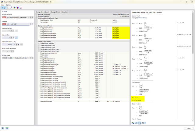
Obliczenia stanu granicznego użytkowalności są w pełni zintegrowane z tabelami wyników w rozszerzeniu Projektowanie konstrukcji drewnianych. Aby sprawdzić wyniki obliczeń, można otworzyć program i wyświetlić wyniki ze wszystkimi szczegółami w każdym miejscu obliczanych prętów. Ponadto dostępne są grafiki z wykresami wyników i stopni wykorzystania.
Cechą szczególną jest to, że Wszystkie tabele wyników i grafiki można zintegrować z globalnym protokołem wydruku programu RFEM/RSTAB jako część wyników wymiarowania drewna. Odkształcenia całej konstrukcji można również wyświetlać i dokumentować w ramach funkcji programu RFEM/RSTAB. Ta funkcja jest niezależna od rozszerzenia.

- 002133
- Ogólne informacje
- Projektowanie konstrukcji drewnianych RFEM 6
- Projektowanie konstrukcji drewnianych RSTAB 9
- Szeroki wybór przekrojów, takich jak przekroje prostokątne, kwadratowe, teowe, okrągłe, złożone, nieregularne przekroje parametryczne i wiele innych (przydatność do obliczeń zależy od wybranej normy)
- Wymiarowanie drewna klejonego krzyżowo (CLT)
- Wymiarowanie materiałów drewnopochodnych i drewna klejonego warstwowo zgodnie z EC 5
- Wymiarowanie prętów o zmiennym przekroju (metoda zgodna z normą)
- Możliwe jest dostosowanie istotnych współczynników obliczeniowych i parametrów normowych
- Elastyczność dzięki szczegółowym opcjom ustawień dla podstawy i zakresu obliczeń
- Szybkie i przejrzyste wyświetlanie wyników dla globalnej oceny ich rozkładu na konstrukcji po zakończeniu obliczeń
- Szczegółowe wyniki obliczeń i niezbędne wzory (jasna i łatwa do zweryfikowania ścieżka wyników)
- Przejrzyste zestawienie wyników w formie numerycznej w stosownych oknach oraz możliwość ich graficznego przedstawienia na konstrukcji
- Integracja wyników z protokołem wydruku programu RFEM/RSTAB
- 002134
- Ogólne informacje
- Projektowanie konstrukcji drewnianych RFEM 6
- Projektowanie konstrukcji drewnianych RSTAB 9
- Wymiarowanie elementów rozciąganych, ściskanych, zginanych, ścinanych, skręcanych i poddanych połączonemu działaniu tych sił wewnętrznych
- Uwzględnienie podcięcia
- Obliczanie ściskania prostopadle do włókien na podporach końcowych i pośrednich z (EC 5) i bez elementów wzmacniających (śruby z pełnym gwintem)
- Opcjonalna redukcja siły tnącej na podporze
- Wymiarowanie prętów zakrzywionych i zbieżnych
- Uwzględnianie wyższych wytrzymałości dla podobnych elementów, które znajdują się blisko siebie (współczynnik ksys wg EN 1995-1-1, 6.6(1)-(3))
- Możliwość zwiększenia nośności na ścinanie dla drewna iglastego zgodnie z DIN EN 1995‑1‑1:NA NDP do 6.1.7(2)
- 002135
- Obliczenia
- Projektowanie konstrukcji drewnianych RFEM 6
- Projektowanie konstrukcji drewnianych RSTAB 9
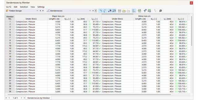
- Analiza stateczności dla wyboczenia giętnego, wyboczenia skrętnego i wyboczenia giętno-skrętnego przy ściskaniu
- Import długości efektywnych z obliczeń przy użyciu rozszerzenia Stateczność konstrukcji
- Graficzne wprowadzanie i kontrola zdefiniowanych podpór węzłowych oraz długości efektywnych w celu analizy stateczności
- Określanie długości zastępczych prętów o zbieżnym przekroju
- Uwzględnienie położenia stężenia zwichrzenia
- Analiza zwichrzenia elementów poddanych obciążeniu momentem
- W zależności od normy istnieje wybór między wprowadzaniem wartości Mcr przez użytkownika, metodą analityczną z normy lub wykorzystaniem wewnętrznego solwera wartości własnych
- Uwzględnienie panelu usztywniającego i ograniczenia obrotu podczas korzystania z solwera wartości własnych
- Graficzne przedstawienie postaci własnej w przypadku zastosowania solwera wartości własnych
- Analiza stateczności elementów konstrukcyjnych ze ściskaniem i naprężeniem zginającym, w zależności od normy obliczeniowej
- Przejrzyste obliczenia wszystkich niezbędnych współczynników, takich jak współczynniki uwzględniające rozkładu momentów lub współczynniki interakcji
- Alternatywne uwzględnienie wszystkich wpływów dla analizy stateczności podczas określania sił wewnętrznych w programie RFEM/RSTAB (analiza drugiego rzędu, imperfekcje, redukcja sztywności, ewentualnie w połączeniu z rozszerzeniem Skręcanie skrępowane (7 stopni swobody))
- 002372
- Ogólne informacje
- Projektowanie konstrukcji drewnianych RFEM 6
- Projektowanie konstrukcji drewnianych RSTAB 9
- Dowolna definicja czasu zwęglania
- W przypadku konstrukcji powierzchniowych (drewno klejone krzyżowo) można obliczyć z przyczepnością lub bez
- Bezpłatna, zdefiniowana przez użytkownika specyfikacja parametrów pożaru
- Uwzględnienie różnych długości efektywnych do obliczania odporności ogniowej
- Opcjonalne obliczenia dla 'ściskania w poprzek włókien'
- Zintegrowane z RFEM/RSTAB graficzne wyświetlanie wyników, np. B. Stopień wykorzystania
- Pełna integracja wyników z protokołem wydruku programu RFEM/RSTAB