101 Wyniki
Wyświetl wyniki:
Sortuj według:
- Proponowane połączenie można zastosować do wszystkich wybranych węzłów w konstrukcji
- Położenie połączenia można zdefiniować w zakładce 'Główne' okna dialogowego rozszerzenia
- Obliczenia są przeprowadzane dla wszystkich połączeń w konstrukcji, a po zakończeniu obliczeń wyniki mogą być wyświetlane we wszystkich połączeniach
- W tabeli wyświetlane są wyniki dla poszczególnych połączeń, każde połączenie jest obliczane i może być zapisane osobno
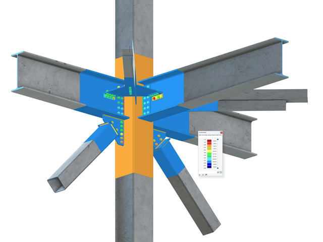
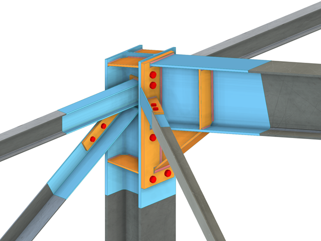
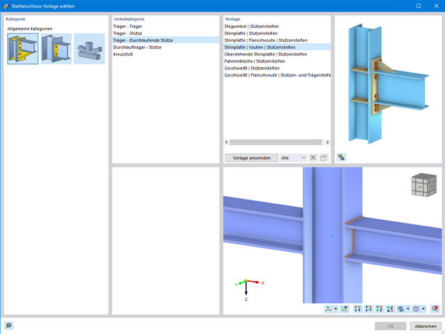
Złożone połączenie belek poziomych ze słupem oraz połączenie stężeń ukośnych
Model połączenia został zamodelowany przy użyciu około 50 komponentów. Model został stworzony na podstawie rzeczywistego przykładu wykorzystania w konstrukcji.
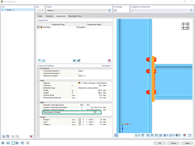
Aby określić nośność śrub na ścinanie, w rozszerzeniu Połączenia stalowe można określić, czy w połączeniu na ścinanie znajduje się trzpień czy gwint.
Przejdź do filmu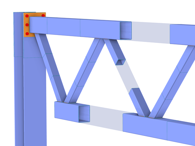
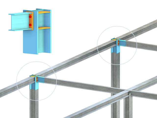
W przypadku przekrojów prostokątnych zwykle można uzyskać bezpośrednie połączenie za pomocą spoin. W ten sam sposób można je jednak połączyć z innymi przekrojami. Ponadto inne elementy, takie jak blachy czołowe, pomagają w łączeniu przekrojów prostokątnych z innymi elementami konstrukcyjnymi.
Stalowe połączenia śrubowe z blachami węzłowymi na konstrukcji zadaszenia.
Pobierz model do analizy statyczno-wytrzymałościowej i otwórz go w programie RFEM 6, korzystając z rozszerzenia Połączenia stalowe.
Wymiarowanie połączenia ramy o prętach zbieżnych i usztywnionych. Dla połączenia przeprowadzono analizę naprężeń i stateczności przy wyboczeniu. Aby wyświetlić wyniki dla wyboczenia, połączenie zostało przekształcone w osobny model.
Rozszerzenie Połączenia stalowe umożliwia wymiarowanie połączeń prętów o złożonych przekrojach. Ponadto można przeprowadzać obliczenia połączeń dla prawie wszystkich przekrojów cienkościennych z biblioteki programu RFEM.
Przejdź do filmuProgram wspiera Cię: Moduł określa siły w śrubach na podstawie modelu analitycznego ES i analizuje je automatycznie. Rozszerzenie przeprowadza obliczenia nośności śrub dla przypadków uszkodzeń, takich jak rozciąganie, ścinanie, docisk otworu i przebicie, zgodnie z normą i wyświetla w przejrzysty sposób wszystkie wymagane współczynniki.
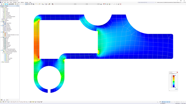
Chcesz przeprowadzić wymiarowanie spoin? Spoiny są modelowane jako sprężysto-plastyczne elementy powierzchniowe, a ich naprężenia są odczytywane z modelu analitycznego ES. Kryterium plastyczności ma reprezentować zniszczenie zgodnie z AISC J2-4, J2-5 (wytrzymałość spoin) i J2-2 (wytrzymałość metalu podstawowego). Obliczenia można przeprowadzić z zastosowaniem częściowych współczynników bezpieczeństwa określonych w załączniku krajowym do normy EN 1993-1-8.
Płyty w połączeniu są wymiarowane w sposób plastyczny poprzez porównanie istniejącego odkształcenia plastycznego z dopuszczalnym odkształceniem plastycznym. Domyślne ustawienie wynosi 5% zgodnie z EN 1993-1-5, Załącznik C, ale można to zmienić według specyfikacji użytkownika, a także 5% dla AISC 360.
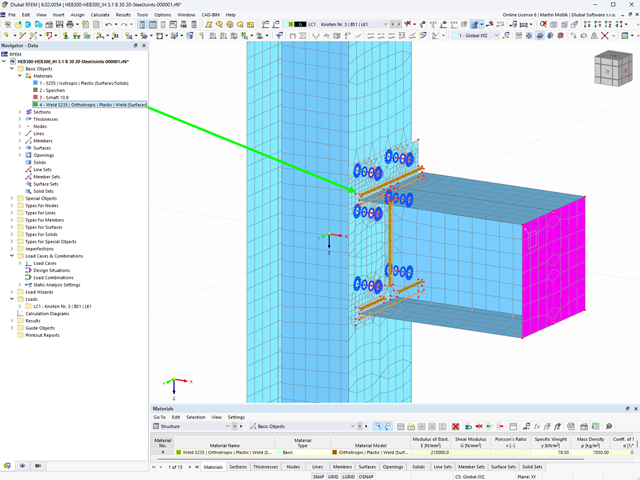
W tym przypadku projektowanie spoin staje się dziecinnie proste. Dzięki specjalnie opracowanemu modelowi materiałowemu „Ortotropowy | Plastyczny | Spoina (Powierzchnie)" można obliczyć wszystkie składowe naprężenia w sposób plastyczny. Naprężenie Tprostopadłe jest również rozpatrywane w sposób plastyczny.
Korzystanie z tego modelu materiałowego umożliwia realistyczne i ekonomiczne projektowanie spoin.
Film wyjaśniający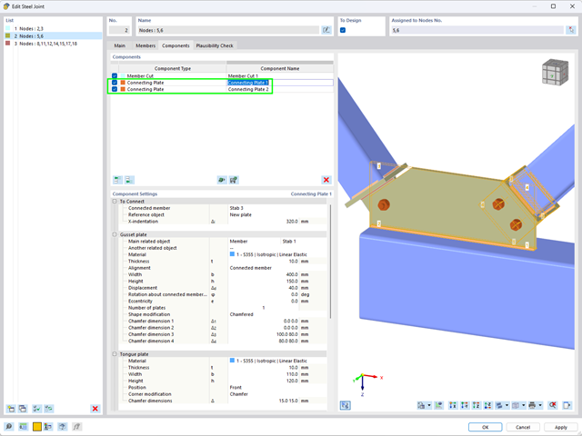
Za pomocą komponentu "Blacha łącząca" można automatycznie utworzyć nową blachę węzłową w rozszerzeniu Połączenia stalowe. Pozwala to na zaoszczędzenie oddzielnych komponentów, a pozostałe elementy, takie jak blacha czołowa i blacha nakładkowa, są automatycznie uwzględniane wraz z wymiarami.
Przejdź do filmu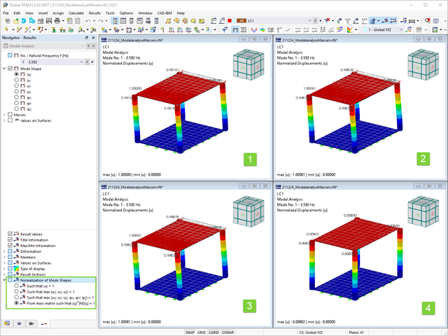
Jak już wiesz, po pomyślnym zakończeniu obliczeń wyniki przypadku obciążenia w Analizie modalnej są wyświetlane w programie. Die erste Eigenform ist für Sie also sofort grafisch oder animiert zu sehen. Dabei können Sie die Darstellung der Eigenformnormierung komfortabel anpassen. Erledigen Sie das am besten direkt im Ergebnisnavigator, wo Sie zur Visualisierung der Eigenformen eine von vier Optionen auswählen:
- Wert des Eigenformvektors uj auf 1 skalieren (berücksichtigt nur die Translationskomponenten)
- Auswahl der maximalen Translationskomponente des Eigenvektors und Einstellung auf 1
- Betrachtung der gesamten Eigenform (inklusive der Rotationskomponenten), Auswahl des Maximums und Einstellung auf 1
- Setzen der modalen Massen mi für jeden Eigenwert auf 1 kg
Ausführlichere Erläuterungen der Normierung der Eigenformen finden Sie hier: Instrukcja online .
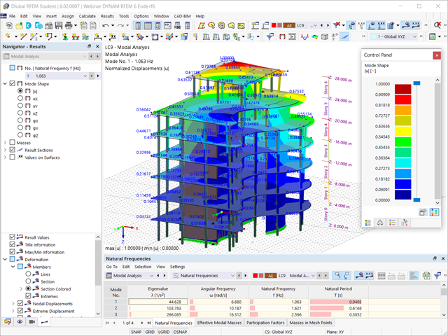
Czy obliczenia się zakończyły? Wyniki analizy modalnej są wówczas dostępne zarówno w formie graficznej, jak i tabelarycznej. Wyświetl tabele wyników dla przypadku obciążenia lub przypadków obciążeń analizy modalnej. Dzięki temu na pierwszy rzut oka można zobaczyć wartości własne, częstotliwości kątowe, częstotliwości i okresy drgań własnych konstrukcji. W przejrzysty sposób wyświetlane są również efektywne masy modalne, modalne współczynniki masy i współczynniki udziału.
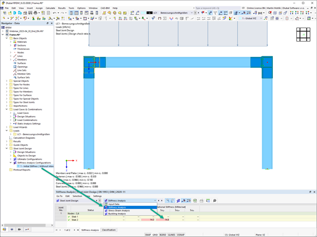
Sztywność początkowa Sj,ini jest parametrem decydującym o ocenie, czy połączenie można scharakteryzować jako sztywne, niesztywne czy przegubowe.
W rozszerzeniu „Połączenia stalowe” można obliczyć początkowe sztywności Sj,ini zgodnie z Eurokodem (EN 1993-1-8 sekcja 5.2.2) i AISC (AISC 360-16 Cl. E3.4) w odniesieniu do sił wewnętrznych N, My i/lub Mz.
Opcjonalne automatyczne przenoszenie sztywności początkowych umożliwia bezpośrednie przenoszenie sztywności przegubowych na końcach prętów w programie RFEM. Następnie cała konstrukcja jest ponownie obliczana, a wynikające z niej siły wewnętrzne są automatycznie uwzględniane jako obciążenia w obliczeniach i wymiarowaniu modeli połączeń.
Ten zautomatyzowany proces iteracji eliminuje konieczność ręcznego eksportu i importu danych, zmniejszając ilość pracy i minimalizując potencjalne źródła błędów.
Film wyjaśniający: Obliczanie sztywności początkowej Sj,ini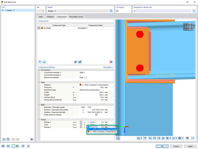
W przypadku spoiny łączącej dwie płyty z różnych materiałów, można teraz wybrać z pola rozwijanego, który z obu materiałów ma zostać użyty do utworzenia spoiny.
Przejdź do filmu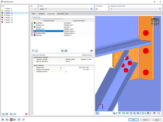
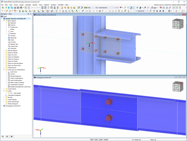
Za pomocą komponentu "Edytor pręta" można modyfikować blachy danego profilu w rozszerzeniu Połączenia stalowe.
Istnieje możliwość zastosowania skosu, fazowania, zaokrąglenia i otworów o wielu kształtach. Obie operacje, "Podcięcie" i "Faza", można wykorzystać dla kilku blach danego profilu.
W ten sposób można fazować na przykład półki dwuteowników (patrz ilustracja).
Przejdź do filmu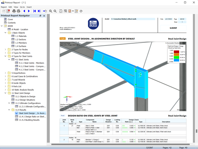
- Wyniki wymiarowania połączeń można wprowadzić do protokołu wydruku
- Podczas tworzenia nowego protokołu wydruku należy wybrać elementy dodane z rozszerzenia Połączenia stalowe
- Za pomocą narzędzia 'Drukowanie grafik do protokołu' można wstawić do protokołu grafikę z wynikami połączenia, w tym z panelem sterowania.
- Protokół wydruku zawiera specyfikacje elementów połączenia, parametry obliczeniowe, wyniki i grafiki
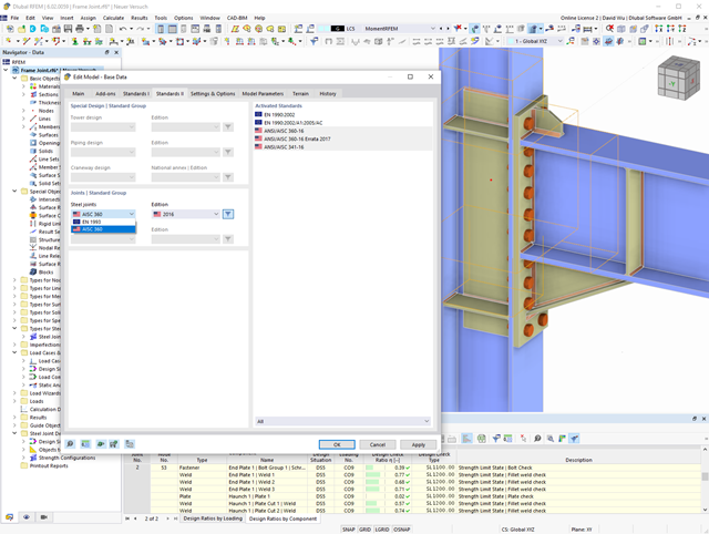
W rozszerzeniu Połączenia stalowe można wymiarować połączenia zgodnie z amerykańską normą ANSI/AISC 360-16. Zintegrowane zostały następujące metody obliczeń:
- Obliczenia współczynnika obciążenia i odporności (LRFD)
- Projektowanie dopuszczalnych naprężeń (ASD)
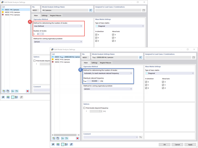
Twoim celem jest określenie liczby postaci drgań własnych? Program oferuje dwie metody. Z jednej strony, można ręcznie zdefiniować liczbę najmniejszych kształtów drgań, które mają zostać obliczone. W tym przypadku liczba dostępnych kształtów postaci zależy od stopni swobody (tzn. liczby punktów mas swobodnych pomnożonych przez liczbę kierunków, w których działają masy). Jest to jednak ograniczone do 9999. Z drugiej strony, maksymalną częstotliwość drgań własnych można ustawić w taki sposób, w jaki program określił kształty automatycznie, aż do osiągnięcia zadanej częstotliwości drgań własnych.
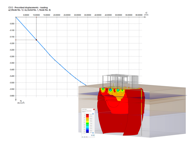
Czy jesteś gotowy na ocenę? Skorzystaj z wykresów obliczeniowych, które pokazują rozkład określonego wyniku podczas obliczeń.
Przypisanie osi pionowej i poziomej wykresu obliczeniowego można dowolnie definiować. Umożliwia to np. wyświetlenie przebiegu osiadania określonego węzła w zależności od obciążenia.
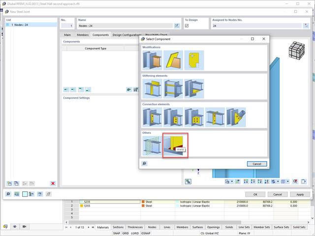
Oprócz innych wstępnie zdefiniowanych elementów w rozszerzeniu Projektowanie połączeń stalowych, do wprowadzania złożonych połączeń można używać podstawowego uniwersalnego elementu 'Spoina ogólna'.
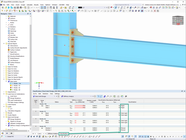
W rozszerzeniu Połączenia stalowe można klasyfikować sztywności połączeń.
Oprócz sztywności początkowej w tabeli wyświetlane są również wartości graniczne dla połączeń przegubowych i sztywnych dla wybranych sił wewnętrznych N, My i/lub Mz. Uzyskana klasyfikacja jest następnie wyświetlana w tabeli jako „przegubowa”, „półsztywna” i „sztywna”.
Przejdź do filmu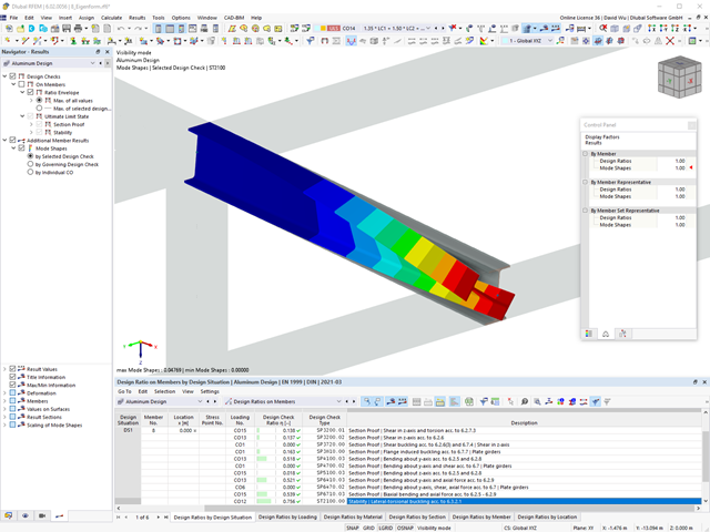
- 002462
- Ogólne informacje
- Projektowanie konstrukcji aluminiowych RFEM 6
- Projektowanie konstrukcji aluminiowych RSTAB 9
Czy do określenia współczynnika obciążenia krytycznego w ramach analizy stateczności użyto dodatkowego solwera wewnętrznych wartości własnych? W takim przypadku można następnie wyświetlić kształt wzorca projektowanego obiektu.
- 002457
- Ogólne informacje
- Projektowanie konstrukcji aluminiowych RFEM 6
- Projektowanie konstrukcji aluminiowych RSTAB 9
Rozszerzenie Projektowanie konstrukcji aluminiowych oferuje dodatkowe opcje. W tym miejscu można również obliczać przekroje ogólne, które nie są wstępnie zdefiniowane w bibliotece przekrojów. Na przykład, utwórz przekrój w programie RSECTION, a następnie zaimportuj go do RFEM/RSTAB. W zależności od zastosowanej normy projektowej dostępne są różne formaty obliczeń. Obejmuje to na przykład równoważną analizę naprężeń.
Ist zudem eine Lizenz für RSECTION und „Effektive Querschnitte“ vorhanden, so können Sie die Nachweise auch unter Berücksichtigung der effektiven Querschnittswerte nach EN 1999-1-1 führen.
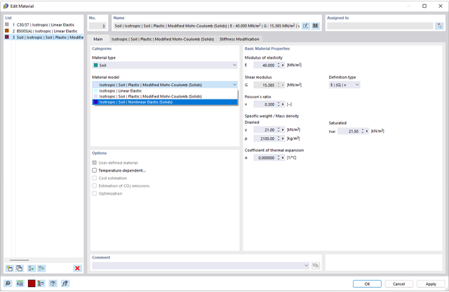
Czy chcesz modelować i analizować zachowanie bryły gruntowej? Aby to zapewnić, w programie RFEM zaimplementowano odpowiednie modele materiałowe.
Można użyć zmodyfikowanego modelu Mohra-Coulomba z liniowo-sprężystym modelem idealnie plastycznym lub nieliniowo sprężystym modelem z edometryczną relacją naprężenie-odkształcenie. Kryterium graniczne, które opisuje przejście od obszaru sprężystości do obszaru płynięcia plastycznego, jest zdefiniowane według Mohra-Coulomba.
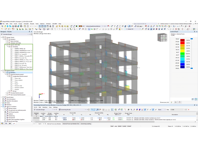
W rozszerzeniu Projektowanie konstrukcji betonowych można przeprowadzać obliczenia sejsmiczne dla prętów żelbetowych zgodnie z EC 8. Są to między innymi następujące funkcje:
- Konfiguracje obliczeń sejsmicznych
- Rozróżnianie klas ciągliwości DCL, DCM, DCH
- Możliwość przeniesienia współczynnika odpowiedzi z analizy dynamicznej
- Sprawdzenie wartości granicznej współczynnika odpowiedzi
- Weryfikacja nośności dla "Wytrzymały słup - słaba belka"
- Uszczegółowienie i reguły szczególne dla współczynnika ciągliwości krzywizny
- Uszczegółowienie i reguły szczególne dla ciągliwości lokalnej
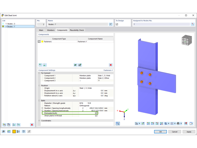
W rozszerzeniu „Połączenia stalowe” można uwzględnić naprężenie wstępne śrub w obliczeniach dla wszystkich komponentów. Sprężenie można łatwo aktywować za pomocą pola wyboru w parametrach śruby i ma ono wpływ zarówno na analizę naprężeniowo-odkształceniową, jak i na analizę sztywności.
Śruby sprężone to specjalne śruby stosowane w konstrukcjach stalowych w celu wygenerowania dużej siły zaciskowej między połączonymi elementami konstrukcyjnymi. Ta siła docisku powoduje tarcie między elementami konstrukcyjnymi, co umożliwia przenoszenie sił.
Funkcjonalność
Śruby sprężane są dokręcane z określonym momentem, co powoduje ich rozciąganie i powstawanie siły rozciągającej. Ta siła rozciągająca jest przenoszona na połączone elementy i prowadzi do powstania dużej siły mocującej. Siła zaciskowa zapobiega poluzowaniu połączenia i zapewnia niezawodne przenoszenie siły.
Zalety
- Wysoka nośność: Śruby wstępnie rozciągane mogą przenosić duże siły.
- Niskie odkształcenie: Minimalizują odkształcenie połączenia.
- Wytrzymałość zmęczeniowa: Są odporne na zmęczenie.
- Łatwość montażu: Są one stosunkowo łatwe w montażu i demontażu.
Analiza i wymiarowanie
Obliczenia śrub sprężanych są przeprowadzane w RFEM z wykorzystaniem modelu analitycznego ES wygenerowanego przez rozszerzenie "Połączenia stalowe". Uwzględnia ona siłę zwarcia, tarcie między elementami konstrukcyjnymi, wytrzymałość śrub na ścinanie oraz nośność elementów konstrukcyjnych. Wymiarowanie odbywa się zgodnie z DIN EN 1993-1-8 (Eurokod 3) lub amerykańską normą ANSI/AISC 360-16. Utworzony model analityczny wraz z wynikami można zapisać i wykorzystać jako niezależny model w programie RFEM.
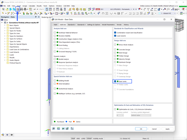
Aby zwymiarować połączenie stalowe, należy aktywować rozszerzenie Połączenia stalowe. Rozszerzenia w programie RFEM 6 są aktywowane w zakładce Rozszerzenia w oknie Edytować model - dane podstawowe. Jeżeli rozszerzenie jest aktywne, jest wyświetlane w nawigatorze.
.png?mw=640&hash=403c565ab80c4dd45c2d1356634fb74a90428b70)
W bibliotece konstrukcji warstwowych dostępni są następujący producenci drewna klejonego krzyżowo:
- Binderholz (USA)
- KLH (USA, CAN)
- Kalesnikoff (USA, CAN)
- Nordic Structures (USA, CAN)
- Mercer Mass Timber
- SmartLam
- Sterling Structural
- Konstrukcje nośne wymienione w Lignatec wydanie 32 "Drewno klejone krzyżowo z produkcji szwajcarskiej"
Wczytanie konstrukcji z biblioteki konstrukcji warstw powoduje automatyczne przejęcie wszystkich istotnych parametrów. Biblioteka jest stale aktualizowana.
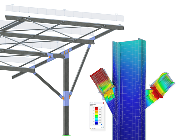
W przypadku elementów połączenia można sprawdzić, czy utrata stateczności jest istotna. Wymaga to rozszerzenia Stateczność konstrukcji.
Współczynnik obciążenia krytycznego obliczany jest dla wszystkich analizowanych kombinacji obciążeń oraz wybranej liczby postaci własnych dla modelu połączenia. Porównaj najmniejszy współczynnik obciążenia krytycznego z wartością graniczną 15 z normy EN 1993-1-1, rozdz. 5. Ponadto użytkownik może samodzielnie dostosować wartość graniczną. Wynikiem analizy stateczności jest wyświetlenie w programie graficznej postaci odpowiednich postaci drgań.
Na potrzeby analizy stateczności dostosowany model powierzchniowy jest wykorzystywany w programie RFEM do rozpoznania lokalnych kształtów wyboczeniowych. Można również zapisać model analizy stateczności wraz z wynikami i wykorzystać jako osobny plik modelu.

W porównaniu z modułem dodatkowym RF-SOILIN (RFEM 5) do rozszerzenia Analiza geotechniczna dla programu RFEM 6 dodano następujące nowe funkcje:
- Tworzenie warstwowego gruntu jako modelu 3D z całości zdefiniowanych próbek gruntu
- Symulacja gruntu zgodnie z teorią Mohra-Coulomba
- Graficzne i tabelaryczne przedstawienie naprężeń i odkształceń na dowolnej głębokości gruntu
- Optymalne uwzględnienie interakcji gruntu i konstrukcji na podstawie modelu ogólnego