81 Wyniki
Wyświetl wyniki:
Sortuj według:

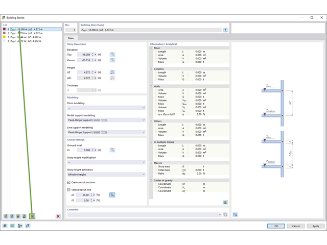
Tabela wyników modelu budynku 'Wyniki według kondygnacji' przedstawia środek ciężkości przypadków obciążeń i kombinacji obciążeń. Oprócz obciążenia stałego uwzględniane są również obciążenia pionowe odpowiednich przypadków obciążeń i kombinacji obciążeń.
W celu wyświetlenia środka ciężkości z uwzględnieniem wybranego obciążenia można również użyć okna dialogowego 'Środek ciężkości oraz Informacje o wybranych obiektach.

W rozszerzeniu Model budynku można zdefiniować właściwości ścian usztywniających i belek-ścian dla odpowiednich rozszerzeń.

Do modelowania kondygnacji, w przypadku płyt można wykorzystać opcję "Tarcza podatna".
Zasadniczo ta opcja modelowania wybiera to samo podejście, co w przypadku modelowania kondygnacji typu "Sztywna przepona". W przeciwieństwie do sztywnej przepony, sprzężenie węzłowe nie jest przeprowadzane od środka ciężkości do każdego węzła ES. W ten sposób możliwe jest uwzględnienie elastyczności płyty.

Podczas generowania ścian usztywniających i belek-ścian można przydzielać nie tylko powierzchnie i komórki, ale także pręty.

W obliczeniach modelu budynku można pominąć otwory o określonej powierzchni. Funkcję tę można aktywować w ustawieniach globalnych kondygnacji budynku. Pojawi się komunikat ostrzegający, że otwory zostały pominięte.
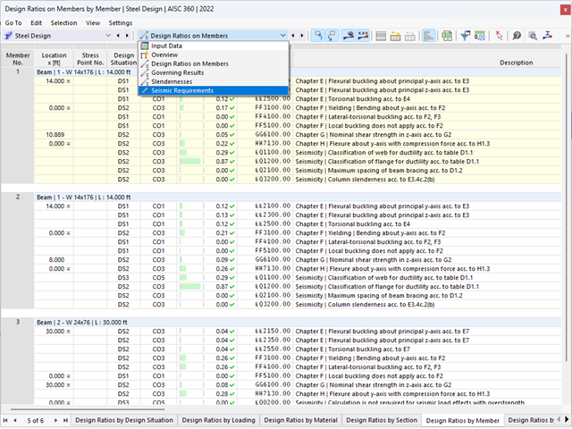
Wynik obliczeń sejsmicznych jest podzielony na dwie sekcje: wymagania dotyczące prętów i połączeń.
"Wymagania sejsmiczne" zawierają Wymaganą wytrzymałość na zginanie i Wymaganą wytrzymałość na ścinanie połączenia belka-słup dla ram sprężystych. Są one wyszczególnione w zakładce 'Połączenia ram momentowych według prętów'. W przypadku ram stężonych w zakładce 'Połączenie stężone według pręta' podawana jest Wymagana wytrzymałość połączenia na rozciąganie oraz Wymagana wytrzymałość połączenia na ściskanie stężeń.
Przeprowadzone kontrole obliczeń są przedstawiane w tabelach. W szczegółach kontroli obliczeń w przejrzysty sposób przedstawione są wzory i odniesienia do normy.
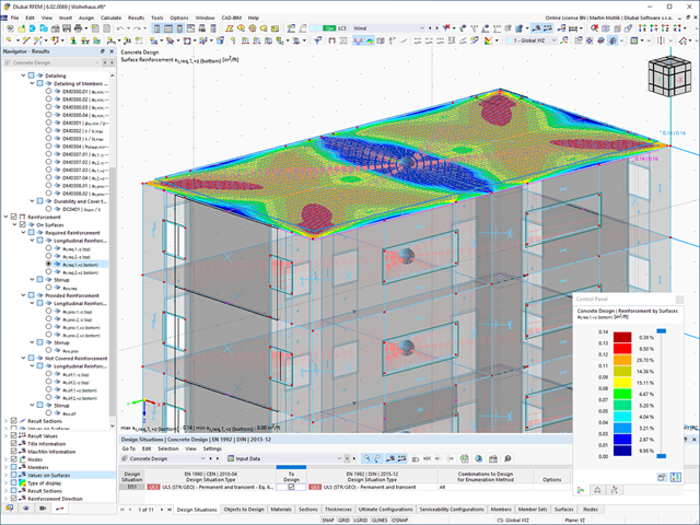
Model budynku jest obliczany w dwóch etapach:
- Globale 3D-Berechnung des Gesamtmodells, in welchem die Decken als starre Ebene (Diaphragma) oder als Biegeplatte modelliert werden
- Lokale 2D-Berechnung der einzelnen Geschossdecken
Die Ergebnisse der Stützen und Wände aus der 3D-Berechnung und die Ergebnisse der Decken aus der 2D-Berechnung werden nach der Berechnung in einem einzigen Modell zusammengefasst. Dadurch muss zwischen dem 3D-Modell und der einzelnen 2D-Modellen der Decken nicht gewechselt werden. Der Anwender arbeitet nur mit einem Model, spart wertvolle Zeit und vermeidet eventuelle Fehler beim händischen Datenaustausch zwischen dem 3D-Modell und der einzelnen 2D-Decken-Modelle.
Die vertikalen Flächen im Modell können vom Nutzer in Schubwände (Shear Walls) und Öffnungsstürze (Sprandels) geteilt werden. Aus diesen Wandobjekten erzeugt das Programm automatisch interne Ergebnisstäbe, so dass diese dann nach der gewünschten Norm im Add-On Betonbemessung für RFEM 6 als Stäbe bemessen werden können.
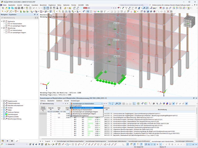
Ściany usztywniające i belki-ściany z modelu budynku są dostępne jako niezależne obiekty w rozszerzeniach. W ten sposób możliwe jest szybsze filtrowanie obiektów w wynikach oraz tworzenie lepszej dokumentacji w raporcie.
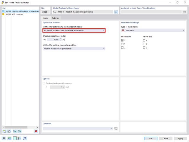
Rozszerzenie Analiza modalna umożliwia automatyczne zwiększanie poszukiwanych wartości własnych do momentu osiągnięcia zdefiniowanego współczynnika efektywnej masy modalnej. Uwzględniane są wszystkie kierunki translacyjne, które zostały aktywowane jako masy do analizy modalnej.
W ten sposób można łatwo obliczyć wymagane 90% efektywnej masy modalnej dla metody spektrum odpowiedzi.
Za pomocą generatora kondygnacji w rozszerzeniu Model budynku można automatycznie tworzyć kondygnacje budynku w zależności od topologii modelu.
- 002733
- Ogólne informacje
- Projektowanie konstrukcji stalowych RFEM 6
- Projektowanie konstrukcji stalowych RSTAB 9
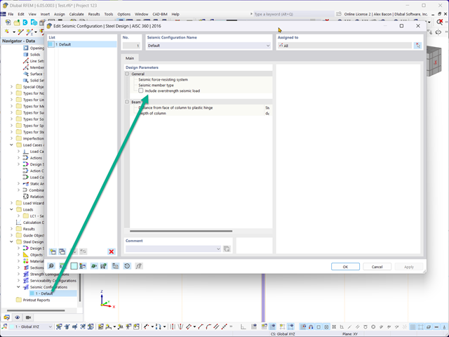
Rozszerzenie Projektowanie konstrukcji stalowych umożliwia przeprowadzanie obliczeń sejsmicznych prętów stalowych zgodnie z AISC 341-16.
W tym celu dostępnych jest pięć typów systemów SFRS (Seismic Force-Resisting Systems).

W przypadku analizy spektrum odpowiedzi modeli budynków można wyświetlić współczynniki wrażliwości dla kierunków poziomych według kondygnacji.
Dzięki tym kluczowym wartościom można zinterpretować wrażliwość na efekty stateczności.
.png?mw=640&hash=403c565ab80c4dd45c2d1356634fb74a90428b70)
W bibliotece konstrukcji warstwowych dostępni są następujący producenci drewna klejonego krzyżowo:
- Binderholz (USA)
- KLH (USA, CAN)
- Kalesnikoff (USA, CAN)
- Nordic Structures (USA, CAN)
- Mercer Mass Timber
- SmartLam
- Sterling Structural
- Konstrukcje nośne wymienione w Lignatec wydanie 32 "Drewno klejone krzyżowo z produkcji szwajcarskiej"
Wczytanie konstrukcji z biblioteki konstrukcji warstw powoduje automatyczne przejęcie wszystkich istotnych parametrów. Biblioteka jest stale aktualizowana.
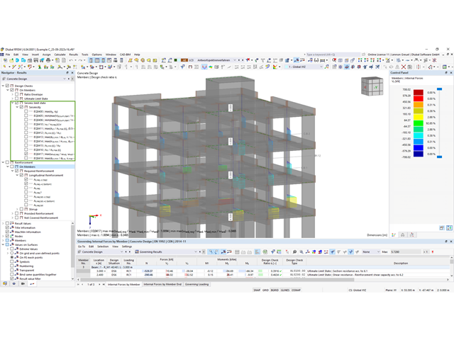
W rozszerzeniu Projektowanie konstrukcji betonowych można przeprowadzać obliczenia sejsmiczne dla prętów żelbetowych zgodnie z EC 8. Są to między innymi następujące funkcje:
- Konfiguracje obliczeń sejsmicznych
- Rozróżnianie klas ciągliwości DCL, DCM, DCH
- Możliwość przeniesienia współczynnika odpowiedzi z analizy dynamicznej
- Sprawdzenie wartości granicznej współczynnika odpowiedzi
- Weryfikacja nośności dla "Wytrzymały słup - słaba belka"
- Uszczegółowienie i reguły szczególne dla współczynnika ciągliwości krzywizny
- Uszczegółowienie i reguły szczególne dla ciągliwości lokalnej
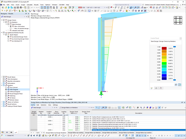
W rozszerzeniu Projektowanie konstrukcji stalowych można przeprowadzić kontrolę obliczeń stateczności i przekrojów profili formowanych na zimno według EN 1993-1-3, zgodnie z punktami 6.1.2 - 6.1.5 i 6.1.8 - 6.1.10.
Przejdź do filmu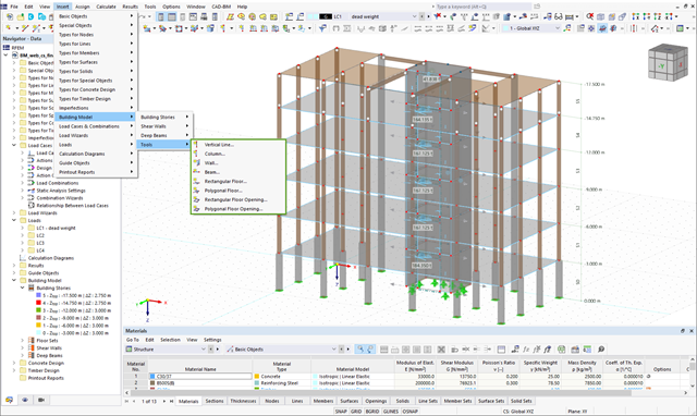
W przypadku elementów w modelach budynków dostępnych jest kilka narzędzi do modelowania:
- Linia pionowa
- Słup
- Ściana
- Belka
- Strop prostokątny
- Płyta wielokątna
- Prostokątny otwór w stropie
- Wielokątny otwór w stropie
Ta funkcja umożliwia definicję elementów na płaszczyźnie podłoża (na przykład z warstwą tła) z powiązanym tworzeniem wielu elementów w przestrzeni.
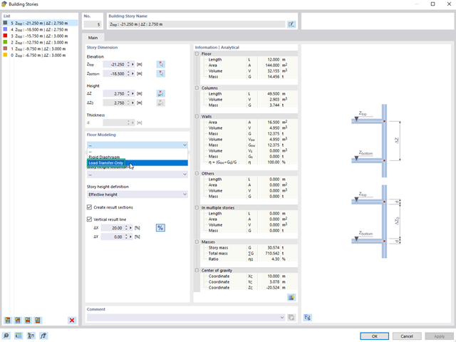
Korzystając z kondygnacji typu "Tylko przenoszenie obciążenia", można uwzględnić w rozszerzeniu Model budynku stropy bez wpływu sztywności do i z płaszczyzny. Ten typ elementu zbiera obciążenia na stropie i przenosi je na elementy nośne modelu 3D. Daje to możliwość symulacji w modelu 3D elementów drugorzędnych, takich jak np. ruszt i inne podobne elementy rozkładu obciążenia, bez dalszych efektów.
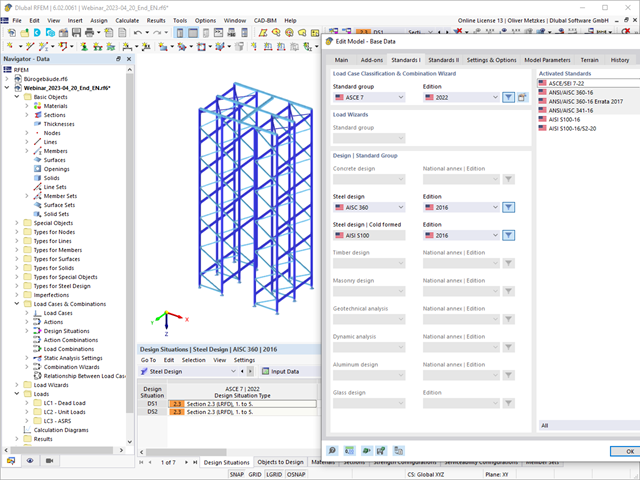
Wymiarowanie prętów stalowych formowanych na zimno zgodnie z AISI S100-16/CSA S136-16 jest dostępne w RFEM 6. Dostęp do obliczeń można uzyskać, wybierając normy „AISC 360” lub „CSA S16” w rozszerzeniu Projektowanie konstrukcji stalowych. Następnie dla obliczeń elementów formowanych na zimno automatycznie wybierane jest „AISI S100” lub „CSA S136”.
Do obliczania sprężystego obciążenia wyboczeniowego pręta program RFEM stosuje metodę DSM. Bezpośrednia metoda wytrzymałości oferuje dwa typy rozwiązań, numeryczne (metoda pasm skończonych) i analityczne (specyfikacja). Krzywą charakterystyczną (sygnaturę) FSM i kształty wyboczenia można wyświetlić w oknie dialogowym Przekroje.
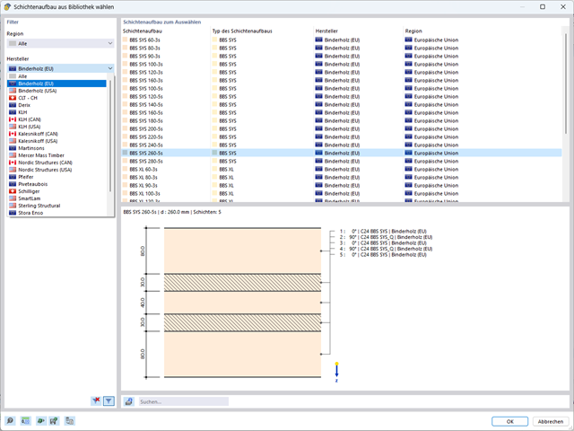
W programie RFEM zaimplementowano bibliotekę płyt z drewna klejonego krzyżowo, z której można importować konstrukcje warstwowe różnych producentów (np. Binderholz, KLH, Piveteaubois, Södra, Züblin Timber, Schilliger, Stora Enso). Oprócz grubości i materiałów warstw podane są również informacje o redukcji sztywności i łączeniu wąskich boków.
Przejdź do filmu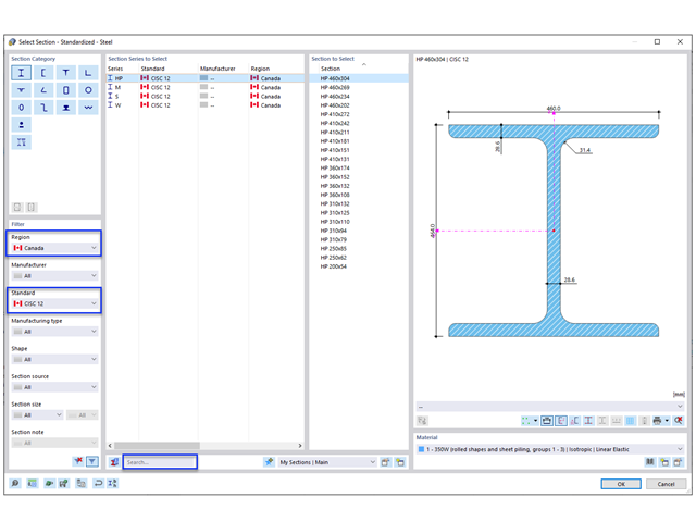
- 002567
- Ogólne informacje
- Projektowanie konstrukcji stalowych RFEM 6
- Projektowanie konstrukcji stalowych RSTAB 9
Nowe przekroje stalowe zgodnie z najnowszą instrukcją CISC (12 wydanie) są dostępne w programie RFEM 6. Przekroje są wymienione w bibliotece Znormalizowane. W filtrze należy wybrać region „Kanada”, a normę „CISC 12”. Alternatywnie nazwę przekroju można wprowadzić bezpośrednio w polu wyszukiwania znajdującym się w dolnej części okna dialogowego.
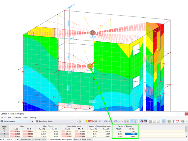
Aktywowałeś rozszerzenie Model budynku ? Bardzo dobrze! Możesz wyświetlić środek sztywności w tabeli i w formie graficznej. Użyj go na przykład do analizy dynamicznej.
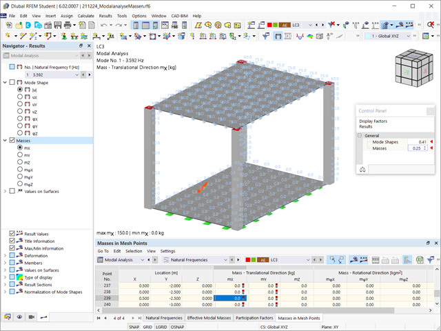
Czy odkryłeś już tabelaryczne i graficzne przedstawianie mas w punktach siatki? Po prawej, jest to również jeden z wyników analizy modalnej w programie RFEM 6. W ten sposób można sprawdzić importowane masy, które zależą od różnych ustawień analizy modalnej. Mogą być one wyświetlane w zakładce Masy w punktach siatki tabeli Wyniki. Tabela zawiera przegląd następujących wyników: Masa - kierunek przesuwny (mX, mY, mZ ), Masa - kierunek obrotowy (mφX, mφY, mφZ ) oraz suma mas. Czy nie byłoby lepiej, gdybyś jak najszybciej przeprowadził ocenę graficzną? Następnie można również wyświetlić graficznie masy w punktach siatki.
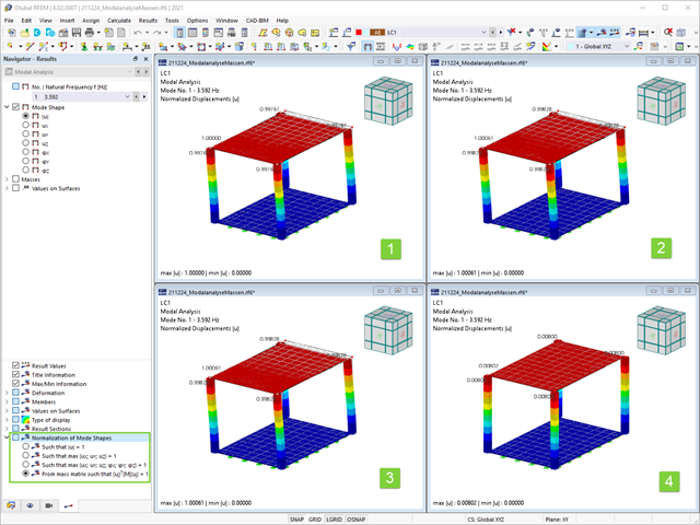
Jak już wiesz, po pomyślnym zakończeniu obliczeń wyniki przypadku obciążenia w Analizie modalnej są wyświetlane w programie. Die erste Eigenform ist für Sie also sofort grafisch oder animiert zu sehen. Dabei können Sie die Darstellung der Eigenformnormierung komfortabel anpassen. Erledigen Sie das am besten direkt im Ergebnisnavigator, wo Sie zur Visualisierung der Eigenformen eine von vier Optionen auswählen:
- Wert des Eigenformvektors uj auf 1 skalieren (berücksichtigt nur die Translationskomponenten)
- Auswahl der maximalen Translationskomponente des Eigenvektors und Einstellung auf 1
- Betrachtung der gesamten Eigenform (inklusive der Rotationskomponenten), Auswahl des Maximums und Einstellung auf 1
- Setzen der modalen Massen mi für jeden Eigenwert auf 1 kg
Ausführlichere Erläuterungen der Normierung der Eigenformen finden Sie hier: Instrukcja online .
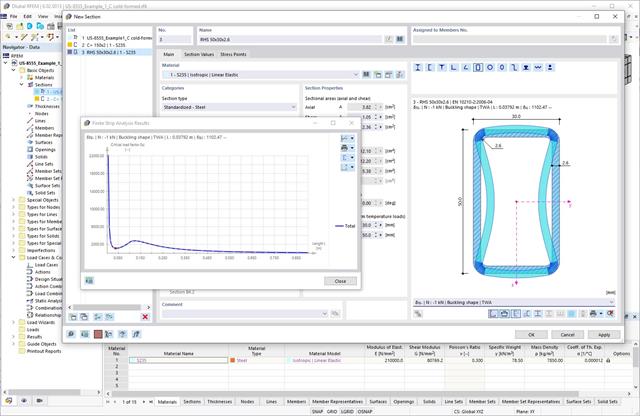
Podczas wymiarowania zgodnie z EN 1993-1-3, możliwe jest przedstawienie graficzne postaci własnej wyboczenia dystorsyjnego przekroju oraz dla przekrojów RSECTION.
Kształt postaci własnej można również wyprowadzić w RSECTION 1 dla przekrojów z biblioteki.
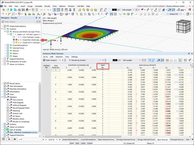
Wyniki naprężeń i odkształceń według powierzchni można wyświetlić w tabeli wyników powierzchni zgodnie z grubością warstwy.
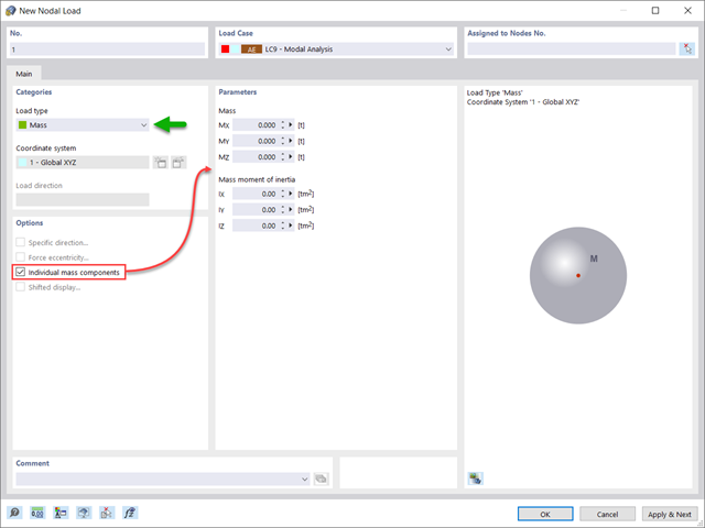
Czy oprócz obciążeń statycznych chcesz uwzględnić również inne obciążenia jako masy? Program umożliwia to dla obciążeń węzłowych, prętowych, liniowych i powierzchniowych. W tym celu podczas definiowania obciążenia należy wybrać typ Obciążenie masą. Dla takich obciążeń należy zdefiniować masę lub składowe masy w kierunkach X, Y i Z. W przypadku mas węzłowych można dodatkowo zdefiniować momenty bezwładności X, Y i Z w celu modelowania bardziej złożonych punktów mas.
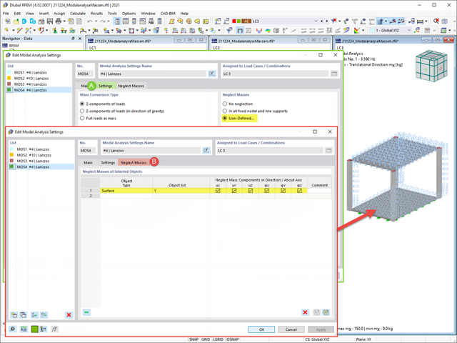
Często zachodzi potrzeba pominięcia mas. Dzieje się tak zwłaszcza w przypadku, gdy wyniki analizy modalnej mają być wykorzystane do analizy sejsmicznej. W tym celu wymagane jest 90% efektywnej masy modalnej w każdym kierunku. Pozwala to na pominięcie masy we wszystkich utwierdzonych podporach węzłowych i liniowych. Program automatycznie dezaktywuje powiązane masy.
Obiekty, których masy mają zostać pominięte w analizie modalnej, można również wybrać ręcznie. Dla lepszego widoku pokazaliśmy to ostatnie na rysunku. W wyniku wyboru przez użytkownika obiektów masowych wraz z skojarzonymi z nimi składowymi masowymi można pominąć masy.
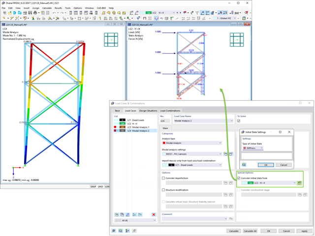
Podczas definiowania danych wejściowych dla przypadku obciążenia analizy modalnej można uwzględnić przypadek obciążenia, którego sztywności reprezentują początkową pozycję analizy modalnej. Jak to zrobić? Jak pokazano na rysunku, należy wybrać opcję "Uwzględnij stan początkowy z". Teraz otwórz okno dialogowe "Ustawienia stanu początkowego" i zdefiniuj typ Sztywność jako stan początkowy. W tym przypadku obciążenia, który jest stanem początkowym branym pod uwagę, można uwzględnić sztywność układu konstrukcyjnego, gdy pręty rozciągane ulegają uszkodzeniu. Celem tego wszystkiego: Sztywność z tego przypadku obciążenia jest uwzględniana w analizie modalnej. W ten sposób uzyskuje się wyraźnie elastyczny system.
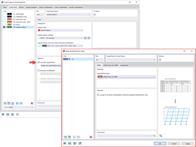
Widać to już na obrazku: Imperfekcje można również uwzględnić podczas definiowania przypadku obciążenia w analizie modalnej. Typy imperfekcji, które mogą być stosowane w analizie modalnej, to obciążenia hipotetyczne z przypadku obciążenia, początkowe przemieszczenie w tabeli, odkształcenie statyczne, postać wyboczeniowa, postać dynamiczna oraz grupa przypadków imperfekcji.
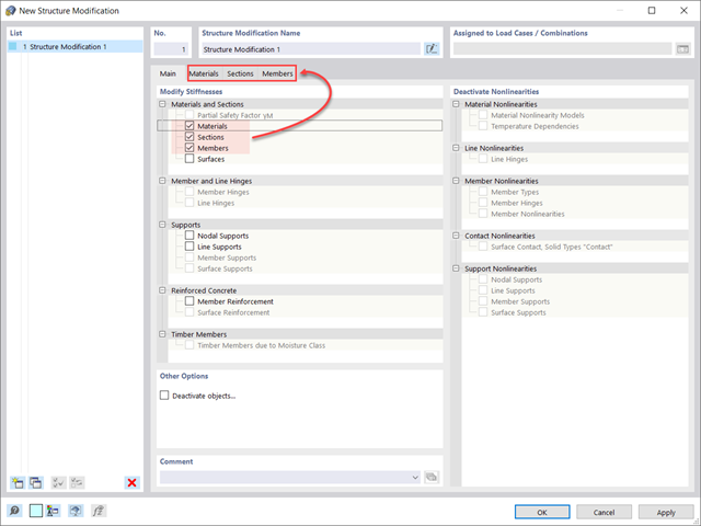
Czy wiecie, że...? W przypadkach obciążeń typu Analiza modalna można z łatwością wprowadzać zmiany konstrukcyjne. Pozwala to na przykład na indywidualne dostosowanie sztywności materiałów, przekrojów, prętów, powierzchni, przegubów i podpór. W przypadku niektórych rozszerzeń można również modyfikować sztywności. Po wybraniu obiektów ich właściwości sztywności są dostosowywane do typu obiektu. W ten sposób można je zdefiniować w osobnych zakładkach.
Czy chcesz przeanalizować uszkodzenie obiektu (na przykład słupa) w analizie modalnej? Jest to również możliwe bez żadnych problemów. Wystarczy przejść do okna Modyfikacja konstrukcji i dezaktywować odpowiednie obiekty.