Material

In the Time-Dependent Properties tab of the Material dialog, you can define the material properties relevant for the time-dependent analysis. In addition to the user-defined input for "Concrete" material types, this is also possible according to standard (EN 1992-1-1).

Settings

In this section, you specify which time-dependent effects and which definition type should be applied. The inputs and the visualization change depending on the selection. To improve clarity, a distinction is made below based on the selection of the definition type.

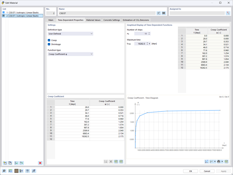
Definition Type: User-Defined

By selecting the definition type User-Defined, the function types Creep coefficient φ and Shrinkage strains ε_cs are available, corresponding to the selection of the applied time-dependent effects Creep and Shrinkage. These can be entered, inserted at the bottom left, or also imported from Excel using the button and exported using the button.

Define Time-Dependent Material Properties - User-Defined Definition Type

Graphical Representation of Time-Dependent Functions

In this section, you can define parameters used for the visualization of the time-dependent functions. The function type selected under Settings determines the time-dependent parameters displayed in the table and the Diagram. The following selection settings are available for the visualization:

• Number of steps: The value n_s influences the division of the graph.
• Concrete age at considered time: The value t represents the endpoint of the abscissa.

Definition Type: According to Standard

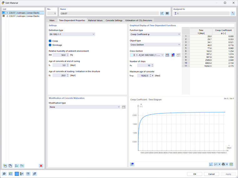
For the definition type According to Standard, the parameters of the time-dependent effects are automatically calculated according to the selected standard. Currently, determination according to "EN 1992-1-1" for concrete is available here. Further information can be found in the manual of the Concrete Design add-on.

Specifying Time‑Dependent Material Properties According to Standard (EN 1992-1-1)

Creep

Select the 'Creep' check box if the time-dependent deformation of the material should be considered in the internal force determination. You can then define the parameters with which the program determines the creep coefficient φ:

• Relative ambient humidity RH
• Concrete age at loading / introduction in the system t₀

Shrinkage

Select the 'Shrinkage' check box if the time-dependent shrinkage strain should be considered as a load. You can then define the parameters with which the program determines the basic drying shrinkage ε_cd,0 and from it the shrinkage strains ε_cs ,ε_ca and ε_cd:

• Relative ambient humidity RH
• Concrete age at end of curing t_s
• Concrete age at loading / introduction in the system t₀

Modification of Concrete Maturation

The following options are available for selection in the list (see image Define time-dependent material properties according to standard):

• None: The concrete ages according to the standard curve.
• Temperature treatment: The temperature treatment affects the hardening of the concrete and thus the effective concrete age at loading. Click the button to define the parameters of the temperature treatment in a separate dialog.
• Measurement of modulus of elasticity: Enter the measured modulus of elasticity E_cm(t) and the time of measurement to consider an equivalent concrete age.
• Measurement of concrete strength: Enter the measured strength f_cm(t) and the time of measurement to consider an equivalent concrete age.

Graphical Representation of Time-Dependent Functions

In this section, you can define parameters used for the visualization of the time-dependent behavior:

• Function type: The function type determines the calculated time-dependent parameters displayed in the table and the Diagram. The following options are available:
  • Creep: Creep coefficient φ at equivalent time
  • Shrinkage: Shrinkage strains ε_cs ,ε_ca and ε_cd
• Object type: The object type for which the visualization is carried out. The following options are available:
  • Thickness
  • Cross-section
• Number of steps: The value n_s influences the division of the graph.
• Concrete age at considered time: The value t represents the endpoint of the abscissa.

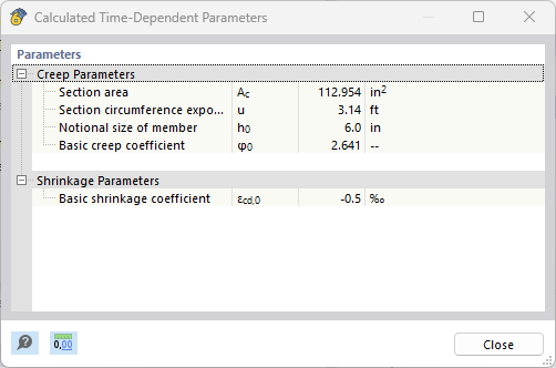
The button below the diagram opens the 'Calculated Time-Dependent Parameters' dialog. There you can read the creep and shrinkage parameters.

Calculated Time-Dependent Parameters

Diagram

In the lower right section, you see the 'Function Value - Time Diagram'. When you move the mouse along the graph, the respective abscissas and ordinates appear. You can zoom with the mouse wheel, move the diagram with the left mouse button, and restore the overall view of the diagram by double-clicking the mouse wheel.

The additional buttons allow you to adjust the display of the diagram and print the graphic.

Display: Linear or Logarithmic

For an optimal display, a linear (lin) and logarithmic (log) division of the axes is possible. The following options are available via the list button :

• lin X / lin Y
• log X / lin Y
• lin X / log Y
• log X / log Y

Print Function

The diagram can also be printed. You have the following options via the list button :

• Print immediately
• To the printout report
• Print in PDF
• Copy to clipboard
• Print as file

Printing graphics is described in the Graphics chapter of the RFEM manual.

Export

You can export the time diagram to Excel using the button.