Modeling Prestressed Bolt Connection

Basics of Joint Diagram

The joint diagram is a graphical representation of forces in a prestressed bolt connection. In this case, the compression forces arising in the components to be connected and the accompanying deformations are contrasted with the forces and deformations in the bolt. Image 01 shows such a diagram.

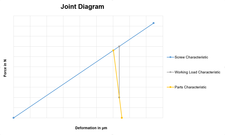
The blue line (characteristic line) represents a graph of the bolt, the yellow one a graph of the structural components. Typically, the bolt stiffness is smaller than the stiffness of the structural components. However, there are also various exceptions such as in the case of nuts. The intersection of both lines represents the preloading force in the connection without an external load applied. The end point of the bolt line is the maximum resistance force in the thread.

In addition to the bolt line and the component line, there is another important characteristic line of the external tensile force (also preload). This line is shown in gray in Image 01. It originates from the characteristic line of the components on the y-axis of the desired residual clamping force. The residual clamping force is the force that still holds the components together. For example, if there is a horizontal force to be absorbed by the connection (without shear strain of the bolt, so only by the component friction) in addition to the tensile component in the case of the existing working load, then the residual clamping force must be selected in a way that there is sufficient resistance.

In addition to these characteristic lines, there are other lines that can be used for a more detailed representation. However, since these lines have no influence on the basic procedure, they will not be explained further in this article, and the presented simplified joint diagram will only be used. For example, the additional characteristic lines would be due to the compression set or the eccentric stress and load.

Formulas of Simplified Joint Diagram

In order to create the joint diagram, it is necessary to calculate the corresponding stiffnesses, deformations, and forces first. In general, the spring stiffnesses can be calculated according to the Hooke's law as follows:

where
c is the stiffness (spring constant),
F is the spring force,
f is the deformation (deflection).

In the case of a tension member with isotropic material, the spring constant can be calculated directly using the elastic modulus (modulus of elasticity):

where
E is the elastic modulus,
A is the cross-section area of ​​the tension member,
l is the length of the tension member.

The bolt stiffness is simplified and only the bolt shaft is applied. Other options are to apply the bolt head, thread, nut, different shaft diameters, and so on. In that case, the elements with their reciprocal value are added to the total stiffness. The spring stiffness of the bolt is calculated using the following formula (Index S):

where
c_S is the spring stiffness of the bolt,
E_S is the elastic modulus of the bolt,
A_S is the cross-section area of ​​the bolt,
l_K is the clamping length (height/thickness of the components).

The thread flank diameter d₃ is used for the cross-section area in the bolt thread range. Thus, the total formula results:

The component stiffness is calculated in a similar way. Since there is one plate or more, the index P is used:

where
c_P is the spring stiffness of the components/plates,
E_P is the elastic modulus of the plates,
A_P is the cross-section area of ​​the plates,
l_K is the clamping length (height/thickness of the components).

The cross-section area A_P depends on the thickness, in contrast to the bolt. It is assumed that the load is extended at an angle of approximately 60°. There are three different cases, as shown in Image 02.

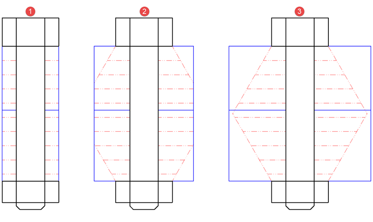
In Case 1, the components between the bolt and the nut are like a sleeve, and this sleeve diameter is maximally equal to the bearing surface diameter of the bolt or nut.
Case 2 covers the range where this sleeve diameter is minimally equal to the bearing surface diameter of the nut or bolt, and maximally equal to the diameter of the load extension cone (marked red in Image 02). This stretches symmetrically from both sides, and the diameter is the largest in the middle of the clamping length.
Case 3 covers the range from the maximum load extension cone to the infinite plate extension. For this reason, it is necessary to calculate the replacement area A_ers. A_ers corresponds to the cross-section area of a replacement cylinder with a constant load extension.

For the following example, Case 3 is sufficient. A_ers is calculated using the following formula (see VDI 2230, edition 1986 [1]):

where
d_W is the bearing surface diameter,
d_h is the bore diameter.

The bearing surface diameter can be applied in a simplified way as 90% of the width across flats:
d_W = 0.9 ∙ s (3.3)
where
s is the width across flats of the bolt head/nut.

Since the load application point in a surface model is not necessarily at the top of the component (the plate), but always in the middle of the surface, the plate stiffness must be determined on this load application point. For this, the load application factor n is introduced, which reduces the clamping length accordingly. This problem is illustrated in Image 03.

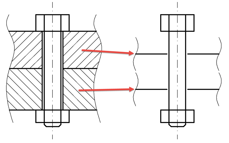
The actual components (two plates, in this case), are reduced to the middle of the surfaces. In the case of two plates, n is always 0.5, as half of each plate is always used. The new plate stiffness c_Pn is then calculated as follows:

where
Φ_K is the load ratio.

To create the characteristic lines, various forces are still required, in addition to stiffnesses. The residual clamping load F_KR, the working load F_A, and the tightening factor α_A (angle-controlled tightening) must be specified. The resulting minimum and maximum assembly forces F_Mmin and F_Mmax, in contrast, must be calculated. Below is the formula for the assembly preloads at an angle-controlled tightening:
F_Mmin = F_Kmin + F_PA (3.6)
F_Mmax = α_A ∙ F_Mmin (3.7)
where
α_A is the tightening factor for the angle-controlled method,
F_Kmin is the minimum required residual clamping force in the connection,
F_PA is the additional plate load due to the working load.

The additional plate load F_PA is the force arising when applying the working load. It is calculated according to the formula:
F_PA = (1 - n ∙ Φ_K) ∙ F_A (3.8)
where
F_A is the working load.

In the simplification without considering settlements, the prestressing force F_V corresponds to the minimum prestressing force F_Mmin. To consider the working load line, the maximum bolt force F_Smax is missing, which arises in the bolt when concerning the working load:
F_Smax = F_Mmax + F_SA (3.9)
where
F_SA is the additional bolt force.

The additional bolt force F_SA is again calculated similarly to Formula 3.8:
F_SA = n∙ Φ_K ∙ F_A (3.10)

The maximum loading capacity of the bolt (F_0.2) as the last missing force must be determined using the cross-section area of the bolt in the thread. This is calculated using the cross-section area diameter d_s, which results from the mean value of the core diameter d_k (d₃) and the flank diameter d_fl (d₂):

where
d₂ is the flank diameter of the thread,
d₃ is the core diameter of the thread,
f_ub is the tensile strength of the bolt material.

In addition to the forces, the deformations must be determined as the corresponding values ​​so the characteristic lines can be entered in the joint diagram. For this, Formula 1.1 converted according to f is used. Below are the formulas for the deformations f to the respective forces F:

This results in the following line points/values ​​for the joint diagram:

Characteristic Line	Deformation	Force
Bolt	0	0
	f0,2	F0,2
Plate	fSMmax	FMmax
	fSMmax + fPMmax or fMmax	0
Working load	fSMmax + fSA	FMmax − FPA
	fSMmax + fSA	FMmax + FSA = FSmax

Table 1 – Line Points/Values ​​for Joint Diagram

Modeling Prestressed Bolt Connection in RFEM

The model should be a good mix of accuracy and practicability. Therefore, the connection will consist of surfaces, members, and contact solids.

The following parameters are specified for the calculation example:
F_A = 25 kN
F_K = 10 kN
E_S = E_P = 210,000 N/mm²
t₁ = t₂ = 10 mm
l_K = t₁ + t₂ = 20 mm
d_h = 10 mm
D_A > d_W + l_K
n = 0.5
α_A = 1.0

Bolt:
M10 8.8
f_ub = 800 N/mm²
d₂ = 9.03 mm
d₃ = 8.16 mm
s = 17 mm

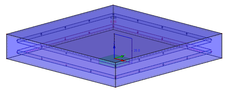
The model includes two superimposed square surfaces with a hole (diameter d_h) in the middle, which have the dimensions 60 x 60 mm (to fulfil D_A > d_W + l_K). Since t₁ = t₂, this results in a plate spacing of 10 mm. The load acts directly in the middle of the plate (neutral fiber). Thus, the resulting n is 0.5. The model is supported by a fixed support at the bottom end of the bolt member. In order to achieve a total support force equal to zero, the load must be applied to both the upper and the bottom plates. The load is 6.95 N/mm² for 25 kN of the total force.

For a good load transfer between the bolt (beam) and plates, a rigid surface (ring) with the outer diameter d_W is modeled around the hole. The connection between the plates is generated using three contact solids. One solid is around the hole without the rigid surface part; two contact solids rest around the hole like two shells. The contact solids must have the same material as the plates to reflect the stiffness between the plates accurately. Furthermore, the contact fails when lifting, and it has a rigid friction in the horizontal direction with the factor of 0.1.

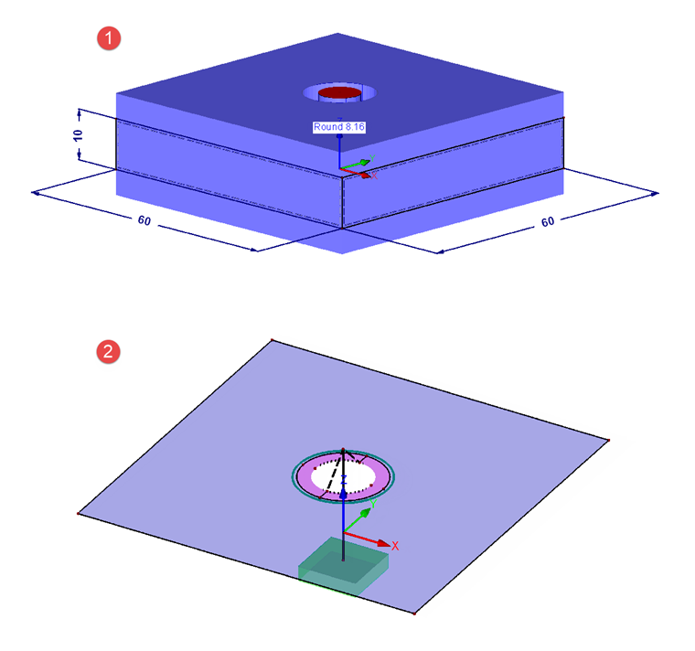
The structure is displayed in Image 04. Number 1 shows the surfaces and members with the actual dimensions. Number 2 shows the upper surface with the beam (bolt) and the rigid members, which represent the connection between the bolt and the plate. The rigid surface (pink) also has a rigid member on the inner edge to be able to transfer any moments.

Another important point is the FE mesh. Due to the small dimensions, the main FE mesh size for l_FE has been set to 2 mm. Moreover, the surface mesh refinement has been defined with l_FE 0.2 mm on the rigid surfaces.

Since neither the bolt diameter nor the working force on the bolt is known in practice, it is possible to model the structure without the hole and to use a rigid member instead of a beam for the first design of the model and for the determination of the bolt forces. This model for pre-dimensioning is shown in Image 05.

In order to be able to detect the residual prestress in the model, a result member was attached parallel to the bolt (distance 0.1 mm). This includes all the internal forces of the contact solid.

Comparison of Analytical and Numerical Solutions

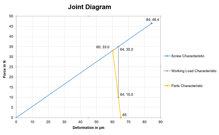
To compare the solutions, it is necessary first to create the joint diagram. The required values are listed in Table 1. The intermediate values and characteristic lines shown in Table 2 are obtained by substituting the values ​​for the practical example (see above). Table 3 includes the summary of the most important values ​​analogous to Table 1, and Image 06 shows the complete joint diagram.

Symbol	Formula Number	Value
cS	2.2	549 kN/mm
Aers	3.2	303 mm²
cP	3.1	3,182 kN/mm
ΦK	3.5	0.147
cPn	3.4	6,921 kN/mm
FSA	3.10	1.8 kN
fSA	4.4	3 μm
FPA	3.8	23.2 kN
FMmax	3.6, 3.7	33.2 kN
fSMmax	4.2	60 μm
fMmax	4.3	65 μm
F0,2	3.11	46.2 kN
f0,2	4.1	84 μm

Table 2 – Intermediate Results and Results of Calculation Example

Characteristic Line	Deformation [μm]	Force [kN]
Bolt	0	0.0
	84	46.2
Plate	60	33.2
	65	33.2
Working load	63	10.0
	63	35.0

Table 3 – Characteristic Line Points/Values ​​of Calculation Example

Two load cases were initially created for the numerical solution. The first load case (LC1 Prestress) includes the member load of the prestress, and the second case (LC2 Working load) includes the working load. Furthermore, the load combination of both load cases (factor 1.0) was generated (CO1: LC1 + LC2). The calculation is based on the linear static analysis with 15 load steps (better convergence in the case of contact solids with failure).

For the prestress, it is possible to apply the member load type initial prestress or end prestress to the member. The actual preload is the end prestress. Since the end prestress load requires a lot of computing time, we recommend using the member load of initial prestress. However, this has the disadvantage that this load does not include the reacting force through the plates. Therefore, the axial force in the member is too small after the calculation, since a part can be reduced by deformation of the plates. This difference can be reduced in two ways. On one hand, this can be predicted by means of the plate deformation and converted into an additional force F_Zus,v (predicted) according to the following formula:
F_Zus,v = f_PMmax ∙ c_S (5.1)

On the other hand, this can also be determined iteratively. For this, the prestress load case must be calculated. The difference between the applied initial prestress and the resulting axial force in the member corresponds to the additional force F_Zus,i (iterative). The following formula can be used:
F_Zus,i = F_Mmax - N_S (5.2)
where
N_S is the axial force in the member at initial prestress F_Mmax.

The additional force F_Zus,v results from the values ​​in Table 2 as follows:
F_Zus,v = f_PMmax ∙ c_S = (f_Mmax - f_SMmax) ∙ c_S = 5 μm ∙ 549kN/mm = 2.8 kN

The iterative additional force F_Zus,i can be obtained after calculating the load case on the member in Image 07.

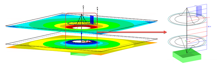
F_Zus,i = 33.2 kN - 30.4 kN = 2.8 kN

Thus, the resulting prestress is 36 kN in both cases. This allows for recalculation of the load case. The result is shown in Image 08.

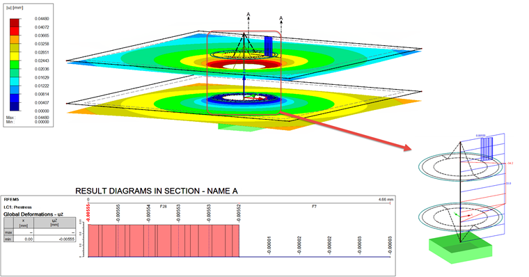
The additional result member, which adds up the contact forces of all contact solids, has the result of 34.2 kN. This is about 1.2 kN more than the axial force of the bolt member, which is 33 kN. The deformation of both surfaces (S1 and S27) shown in the diagram must be added in order to be able to compare it with f_PMmax. On average, this results as follows:

The deformation is thus 0.6 μm greater than the calculated deformation f_Mmax.

The result of the calculations subjected to the working load in LC1 is shown in Image 09.

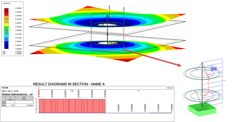
The bolt member has the result of 33.9 kN. This member force can be compared to the force F_Smax = 35 kN (see Table 1 and Table 3, Working Load). The difference is 1.1 kN. The deviation of the differences is also important here. According to the analytical calculation, the difference should be equal to the force F_SA = 1.8 kN. However, the difference of the FE model is only half as great, with 33.9 kN − 33 kN = 0.9 kN.

Similar deviations are obtained in the case of deformation (see the diagram in Image 09). The value shown is the value reduced by the working load. Thus, the deformation must be calculated by the working load using the deformation by the prestress. The actual deformation is the difference between u_z,1 and the mean deformation in the diagram. The analytical reference value is f_SA. This results in the deformation u_z,2:

Thus, the deformation is about 1.4 μm smaller than the calculated deformation f_Mmax.

Finally, the results in the result member are compared. As you can see in Image 09, the load for the result member is the compressive force of 10.6 kN. This value must be compared with the clamping load F_K = 10 kN. This results in a deviation of 0.6 kN. Table 4 includes a summary of all the results.

Symbol	Analytical Value	FEM Calculation		Deviation
		Member	Plate
FMmax [kN]	33.2	33.0	34.2	0.2 / 1.2
fPMmax [μm]	5.0	-	5.6	0.6
fSA [μm]	3.0	-	1.6	1.4
FMmax + FSA [kN]	35.0	33.9	-	1.1
FMmax - FPA [kN]	10.0	-	10.6	0.6

Table 4 – Comparison Values of Analytical Model/FEM Calculation

Evaluation

As shown in Table 4, there are partially large differences between the models. Generally, the largest matches are in the Prestress load case. Depending on the evaluation of the result member (plate) or the bolt member, the deviations from F_Mmax are 3.6% or 0.6% (referred to the analytical result).

The largest deviation is the result of the bolt member and the plate deformation after applying the working load. In this case, there is a deviation of 1.1 kN between the axial force on the member and the analytical solution. This deviation, referred to the analytical solution, is initially 3%. However, the difference is much greater when referred to the bolt additional force. The deviation of the FEA model is as follows:
F_SA,FEM = (F_Mmax + F_SA) - F_Mmax = 33.9 kN - 33 kN = 0.9 kN << 1.8 kN = F_SA

These deviations can be caused by the fact that both plates have no rigidity in the z-direction and the contact solid has only one FE element in its thickness. Thus, there can be no load extension within the solid. The load transfer in the solid is done exclusively via the deformation of the plate by bending and shear force. It is obvious from the values that the FE model in the Prestress load case in the combination of plates and contact solids has smaller stiffness than in the analytical model (see the smaller deformation). At this point, the higher stiffness of the bolt can be excluded, as this is determined by the beam theory and the cross-section.

On the other hand, there is a smaller deformation in the case of the load combination in the FEA model, or the bolt force has a significantly smaller increment. This, again, indicates the higher stiffness in the plate. In summary, there is only one explanation for this: The composite of a plate and contact solids has a different load extension, so the approach from Formula 3.2 in the FEA model is not valid in the form. It would likely be necessary to examine a real example or an extended FEA model to find out which solution is closer to reality.

However, it is important to note the following: The residual clamping force is almost identical in both variants. Thus, the prestress in the connection is modeled well and can be used for the joint analysis.

Summary

Modeling a prestressed bolt connection using contact solids, surfaces, and beams is a combination of a practical solution and real display. Practical means that the computing time is significantly smaller, compared to the calculation with FEA solids, which would probably represent the connection more accurately. However, it is necessary to improve the bolt design or to perform further analysis, which sets the results in relation with the reality.

Since the preloading forces and the residual clamping forces largely correspond to those from the analytical calculation, it can be assumed that this modeling type can be used for the connection analysis.

Literature

[1]	Association of German Engineers: (1986). Guideline VDI 2230 – Systematic Calculation of Highly Stressed Bolted Joints. Berlin: Beuth.