123x

002071

Dr. rer. nat. Marc Gebhardt

2026-08-12

From Analytical Creep Curve, Through Rheological Model, to Time-Dependent Strain State

This article aims to clearly explain, using a simplified example, the theoretical background and implementation of time-dependent creep analysis in RFEM 6.

Introduction

If a structural component is subjected to a constant load (stress \(\sigma = \text{constant}\)) over a long period of time, additional time-dependent creep strain \(\varepsilon(t)\) occurs in addition to the immediate elastic deformation. This is particularly relevant for structural components made of concrete and timber. This effect can be taken into account in a simplified manner by reducing the modulus of elasticity. For a much more accurate analysis, however, a time-incremental calculation should be performed using a rheological model—in this case, the Kelvin chain model. This allows you to consider redistribution effects in the structural system and material nonlinearities. By recalculating the stiffness at each time step, it is thus possible to analyze more realistic structural behavior and, for example, to model construction stages and the mutual influence of structural elements. Further information can be found at the following links:

Model Description and Creep Coefficient Determination According to Eurocode 2

A simple model was created to compare and demonstrate the analysis options in RFEM 6. This model consists of a 1 m long, simply supported column with a rectangular cross-section and an edge length of 100 mm. C25/30 was selected as the material. The load consists of a compressive force of 100 kN at the top of the column. The model is shown in the image below and can be downloaded via the link provided.

The analytical creep curve is taken from EN 1992-1-1, Annex B, and can be calculated using the following formula. It gives the ratio of creep strain to elastic strain.

φ (t, t_{0}) = \frac{ε_{c r}}{ε_{e l}} = \frac{ε_{c} (t) - ε_{c 0}}{ε_{c 0}} = φ_{0} \cdot {(\frac{t - t_{0}}{β_{H} + (t - t_{0})})}^{0, 3}

φ(t,t0)	Creep coefficient
εcr	Creep strain
εel	Elastic strain
εc(t)	Strain of concrete over time
εc0	Immediate strain of concrete
φ0	Creep basic value
βH	Coefficient for considering relative humidity and the effective thickness of the building component

Creep Coefficient According to EN 1992-1-1, Annex B

The total strain at any given time can be calculated using the following formula.

ε_{c} (t) = ε_{c 0} \cdot (1 + φ (t, t_{0})) = \frac{σ_{0}}{E_{c m}} \cdot (1 + φ (t, t_{0}))

εc(t)	Strain of concrete over time
εc0	Immediate strain of concrete
φ(t,t0)	Creep coefficient
σ0	Stress (constant)
Ecm	Mean modulus of elasticity of concrete

Total Strain (Creep Coefficient)

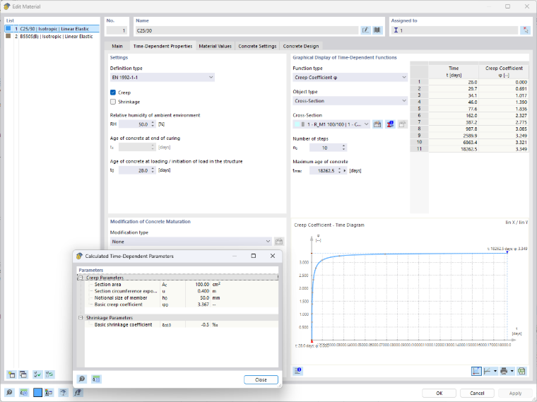
In RFEM 6, you can perform the calculation using intermediate values in the “Edit Material” dialog box under the “Time-Dependent Parameters” tab and check it for the selected cross-section or thickness at logarithmically distributed control points. Further control and visualization are available using the “Advanced Time-Dependent Properties of Concrete” option in the “Edit Cross-Section” and “Edit Thickness” dialog boxes. The following link to the manual provides more details on this, and the image below shows the values for the cross-section used here.

Online Manuals RFEM 6 | Time-Dependent Analysis (TDA) | Input | Material

KB 2071 | Time-dependent properties in the Material dialog box

KB 2071 | Time-Dependent Properties in Material Dialog Box

Rheological Model

Kelvin Chain Model

For the time-dependent analysis of creep behavior, the Kelvin chain model is implemented as a rheological model in RFEM 6. In this Kelvin chain, Kelvin-Voigt elements with a free spring E₀ and an optional free damper η_∞ are connected in series. The free spring is responsible for the immediate strain, which corresponds to the result of a normal structural analysis. The free damper—which would lead to a strain component that continues to increase endlessly—is omitted due to its irrelevance for materials typically used in construction. A Kelvin-Voigt element consists of a spring element and a damper element connected in parallel. This is shown schematically in the following image:

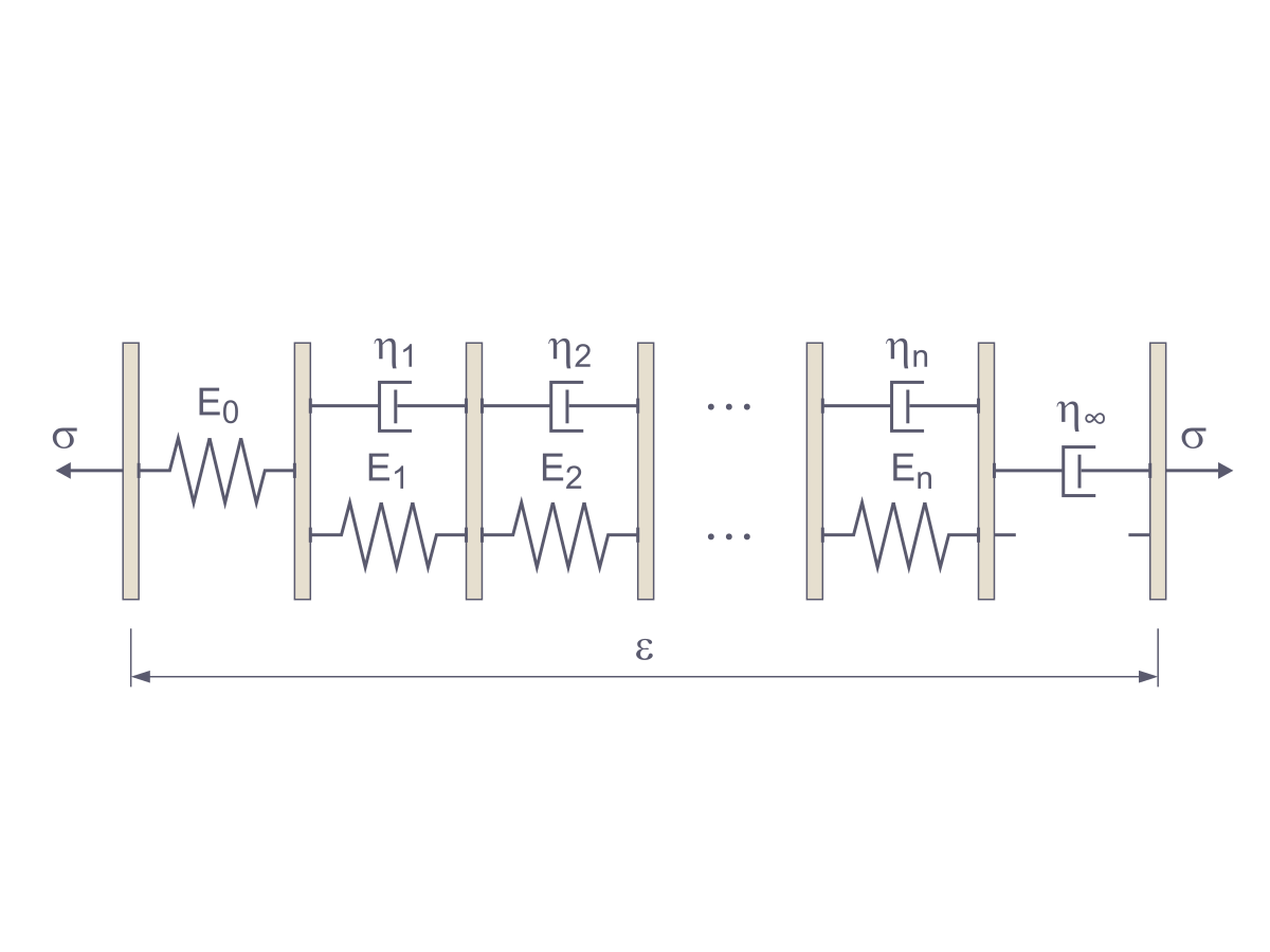
Generalized Kelvin-Voigt Chain Model

The total creep function of the Kelvin chain results from the summation of the components of the elements connected in series. It describes the strain behavior with respect to the applied stress over time. The Kelvin-Voigt elements thus have two adjustable variables: the stiffness E_k and the delay time 𝜏_k. The latter, in turn, is calculated as the dynamic viscosity divided by the stiffness.

J (t) = \frac{ε (t)}{σ} = \frac{1}{E_{0}} + \sum_{k = 1}^{n} \frac{1}{E_{k}} (1 - e^{- \frac{t}{τ_{k}}}) + \frac{t}{η_{∞}}

ε	Strain
t	Time
σ	Stress
E0	Modulus of elasticity of the free spring (immediate strain)
k	Current element
n	Number of elements
Ek	Modulus of elasticity of the current element
e	Euler's number
τk=ηk/Ek	Delay time of the current element
η∞	Dynamic viscosity of the free damper (Newtonian fluid)

Generalized Kelvin Chain Model – Total Strain

Adaptation to Analytical Creep Behavior

The Kelvin-Voigt elements are adapted by minimizing the square of the difference between their creep coefficient components and those of the analytical solution.

min_{α_{k}} \sum_{i = 1}^{m} {(φ (t_{i}) - φ_{∞} \sum_{k = 1}^{n} α_{k} (1 - e^{- t_{i} / τ_{k}}))}^{2}

αk	Weight factor (conditions: greater than 0, and their sum must equal 1)
i	Time increment
m	Number of time increments
φ(ti)	Creep coefficient at time i
φ∞	Creep coefficient (infinite)
k	Current element
n	Number of elements
e	Euler's number
ti	Time at time i
τk=ηk/Ek	Delay time of the current element

Adjustment of Creep Coefficient Prony Series

To visualize this, a least-squares adjustment was performed using a script for different numbers of Kelvin chain elements. The image below on the left shows a comparison of Kelvin chains with 1, 3, 5, and 10 elements with the analytical creep function and the control points taken from RFEM 6. As you can see here, increasing the number of elements also reduces the maximum deviation. Of course, this is associated with increased computational effort. Sufficient accuracy was already achieved with just 5 Kelvin-Voigt elements without any special weighting.

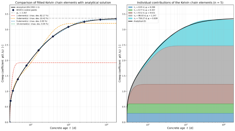
KB 2071 | Creep Coefficient over Time

For simplicity, the delay times can be regarded as the point in time at which the corresponding element begins to contribute to the creep behavior. The following table shows these components for a 5-element Kelvin chain, showing the components for the final creep coefficient based on the components of the individual elements. The creep coefficient can be estimated using the following formula.

φ_{a p p} (t) = \sum_{k = 1}^{n} φ_{k} \cdot (1 - e^{- (t - t_{0}) / τ_{k}})

φ(app)	Approximated creep coefficient at time t
φk	Creep coefficient of the element k
k	Current element
n	Number of elements
e	Euler's number
ti	Current time
t0	Time of loading start
τk=ηk/Ek	Delay time of the current element

Approximated Creep Coefficient

Delay Times, Stiffnesses, and Creep Modulus Contributions of Kelvin Chain with 5 Elements
No.	τ_k [d]	E_k [MPa]	φ_k [—]	Component [%]
1	0.05	107,683	0.2879	8.7
2	0.77	101,086	0.3067	9.3
3	8.52	49,094	0.6314	19.1
4	86.83	24,862	1.2469	37.6
5	759.2	36,940	0.8392	25.3
Total	—	—	3.3121	100.0

Time-Incremental Calculation of Creep Behavior

In the example presented here, the creep behavior was analyzed by dividing the time into 10 linearly distributed time increments. Thus, a state is calculated every 1,823.5 days. In the first step, the initial strain is determined to be 0.323. This is followed by the first time increment from 28 days (loading start) to day 1,851.5. The image below shows a comparison of the incremental calculation using RFEM and the analytical solution on the left. In the diagram on the right, the strain components for a Kelvin chain with 5 elements are displayed as a stacked plot, similar to the previous image.

KB 2071 | Strain Diagram over Time

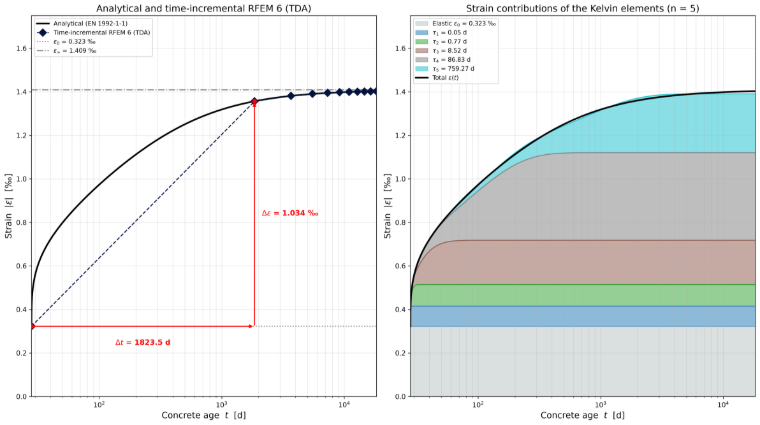
The following table shows the results of the time-incremental calculation. Based on a simplified linear approach to creep behavior using the reduction of the modulus of elasticity, an effective modulus of elasticity per time increment can also be determined in this simple example. Thus, in the first step, the logarithmic nature of the underlying function already results in a reduction of approximately 76%. The reduction, using a final creep factor of 3.349, leads to a 77% reduction to 7126 MPa.

E_{c, e f f, t} = \frac{σ}{ε (t)} = \frac{E_{c m}}{1 + φ (t, t_{0})}

Ec,eff,t	Effective modulus of elasticity of the concrete
Ecm	Average modulus of elasticity of concrete
φ(t,t0)	Creep coefficient at time t, related to the initial time

Effective Modulus of Elasticity at Time t

Strain over Time
Step	t [d]	Δt [d]	ε [‰]	Δε [‰]	E_eff [MPa]	ΔE_eff [MPa]
0	28.0	0.0	0.323	0.000	30999	0
1	1851.5	1823.5	1.356	1.034	7373	-23626
2	3674.9	1823.4	1.381	0.025	7241	-132
3	5498.4	1823.5	1.391	0.010	7190	-51
4	7321.8	1823.4	1.396	0.005	7166	-24
5	9145.3	1823.5	1.398	0.002	7154	-12
6	10968.7	1823.4	1.399	0.001	7146	-8
7	12792.1	1823.4	1.400	0.001	7142	-4
8	14615.6	1823.5	1.401	0.001	7138	-4
9	16439.0	1823.4	1.402	0.001	7134	-3
10	18262.5	1823.5	1.402	0.001	7131	-3

Concluding Remarks

In this simplified example, the time-incremental calculation using the linear creep approach shows no difference when the modulus of elasticity is reduced. However, this cannot be assumed as a general rule. For example, only by using a direct incremental approach based on a rheological model can nonlinear material behavior, component interaction, and changing load conditions and construction stages be correctly taken into account.

Author

Marc works in Product Engineering with a focus on geotechnical engineering and also assists with customer support. He applies his technical expertise to address complex issues.

Links

;