22 Results
View Results:
Sort by:
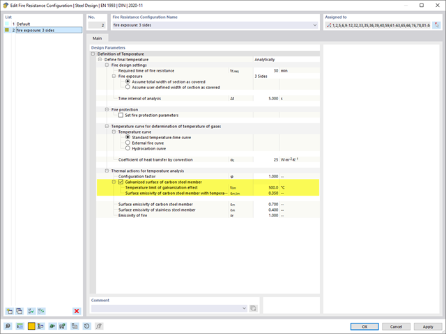
With the Steel Design add-on, you can design structural steel components in the event of fire using the simple design methods according to Eurocode 3. The component temperature at the time of the design check can be determined automatically according to the temperature-time curves specified in the standard. In addition to considering a cladding for fire protection, it is also possible for you to take account of the beneficial properties of hot-dip galvanization.
Steel has poor thermal properties in terms of fire resistance. The thermal expansion for increasing temperature is very high compared to that of other building materials, and might result in effects that were not present in the design at normal temperature due to restraint in the component. As temperature increases, steel ductility increases, whereas its strength decreases. Since steel loses 50% of its strength at temperature of 600 °C, it is important to protect components against fire effects. In the case of protected steel components, the fire resistance duration can be increased due to the improved heating behavior.
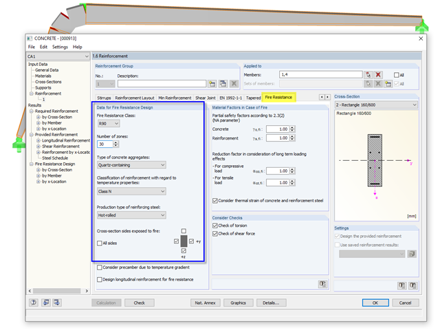
The reinforced concrete design for fire situations is carried out according to the simplified method based on EN 1992-1-2, Clause 4.2. The "zone method" described in Annex B.2 is used: The cross-section is subdivided into a number of parallel zones of equal thickness, and their temperature-dependent compressive strength is determined. The reduced load-bearing capacity in the event of fire exposure is thus represented by a reduced structural component's cross-section with reduced strengths.
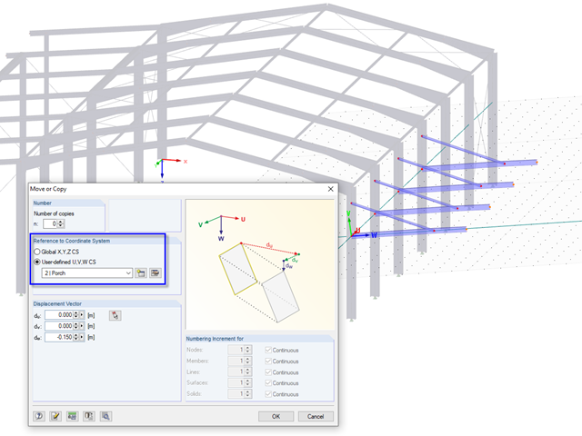
In RFEM and RSTAB, it is possible to move or copy models or parts of the model in a user-defined coordinate system. To use this option, a user-defined coordinate system must be available, of course.
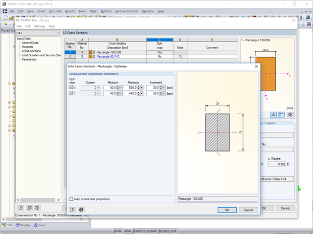
In the course of a reasonable pre-dimensioning of cross-sections, you can optimize the cross-sections of the corresponding section series in the RF‑/TIMBER Pro add-on module.
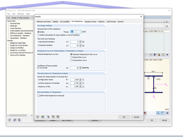
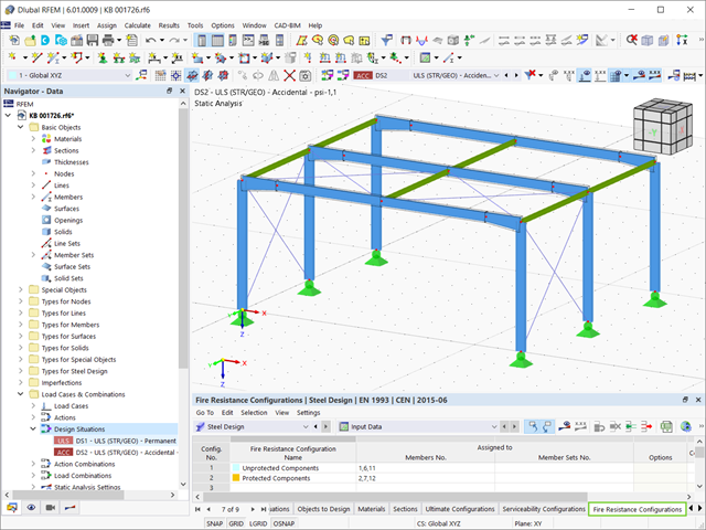
The RF-/STEEL EC3 add‑on module allows for the fire protection design of structural steel components. The simplified analysis is performed by determining the steel temperature iteratively for a particular point of time.
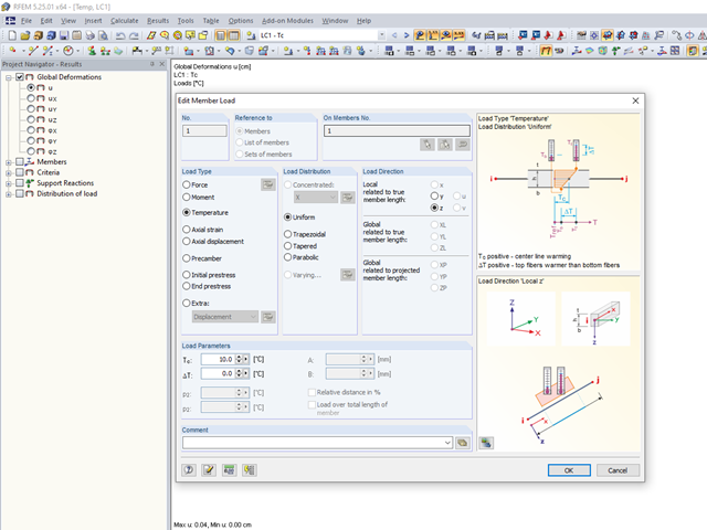
The RFEM and RSTAB structural analysis programs are able to simulate a thermal strain of structural components by means of temperature loads.
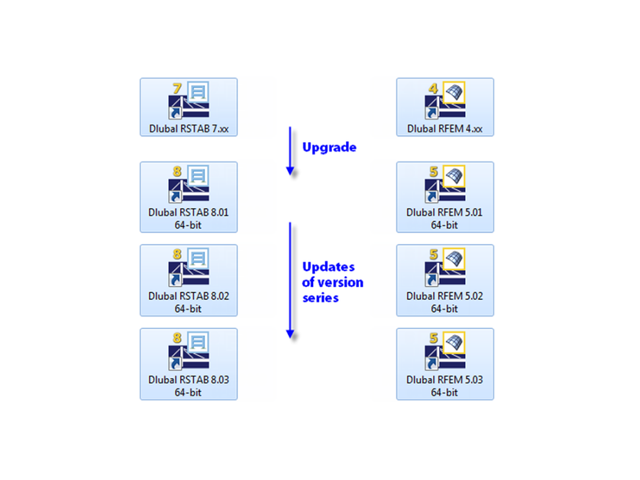
When updating within a version series (for example, RFEM 5.01.01 to 5.01.02), the old program files are removed and replaced by new ones. The project data, of course, remain unchanged. When updating to the next version series (for example, RFEM 5.02.01), the new version is installed in parallel. The program files are located in different directories, so the previous version is still available.
With RF-/STEEL EC3, you can utilize nominal temperature-time curves in RFEM and RSTAB. The standard time-temperature curve (ETK), the external fire curve and the hydrocarbon fire curve are implemented. Moreover, the program provides the option to directly specify the final temperature of steel.
The fire resistance design can be performed according to EN 1993-1-2 in RF-/STEEL EC3. The design is carried out according to the simplified calculation method for the ultimate limit state. Claddings with different physical properties can be selected as fire protection measures. You can select the standard temperature-time curve, the external fire curve, and the hydrocarbon curve to determine the gas temperature.
You can apply nominal temperature‑time curves in RFEM or RSTAB using RF‑/STEEL EC3. For this, the standard time-temperature curve (ETK), the external fire curve and the hydrocarbon fire curve are implemented in the program. Based on these temperature curves, the add‑on module can calculate the temperature in the steel cross‑section and thus perform the fire design using the determined temperatures. This article explains the thermal behavior of structural steel, as this has a direct impact on the calculation of component temperatures in RF‑/STEEL EC3.
![Section Factor Am/V for Unprotected Steel Components (Source: [5])](/en/webimage/009429/2418748/01-en-1-png.png?mw=640&hash=0fa099ecd1abc5310bef76fe3f22b7fe0c925df6)
Using RF-/STEEL EC3, you can apply nominal temperature-time curves in RFEM or RSTAB. For this, the standard time-temperature curve (ETK), the external fire curve, and the hydrocarbon fire curve are implemented in the program. Based on these diagrams, the add-on module can calculate the temperature in the steel cross-section and thus perform the fire design. This article explains the behavior of protected and unprotected steel cross‑sections.
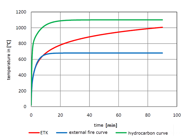
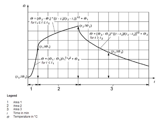
Using RF-/STEEL EC3, you can apply nominal temperature-time curves in RFEM or RSTAB. The standard time-temperature curve (ETK), the external fire curve and the hydrocarbon fire curve are implemented. Moreover, the program provides the option to directly specify the final temperature of steel. This steel temperature can be calculated using the parametric temperature-time curve, as described in the Annex to DIN EN 1992-1-2. The different fire exposures are explained in this article.
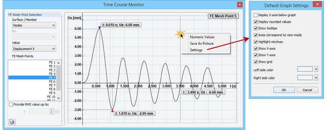
The Time Course Monitor displays the results of a time history analysis from RF‑/DYNAM Pro – Forced Vibrations. The graphic can be adjusted in the settings. This can be reached by right-clicking in the shortcut menu. For example, you can activate or deactivate the grid in the graphic. These changes are transferred to the printout report when you print.
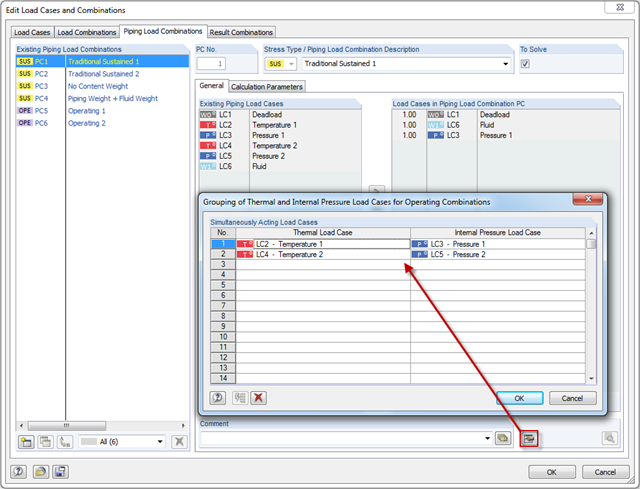
As in RFEM, load combinations can be generated automatically in RF‑PIPING. This feature is activated by default and creates the recommended load and result combinations for piping design. It is necessary to assign the relevant action category to load cases in order to generate the correct combinations. To do this, new action categories have been implemented specifically for loads on piping.
Pressure temperature conditions are generated as the sets of the first (second, third, and so on) load case of the "Pressure" category and the first (second, third, and so on) load case of the "Temperature" category. The default setting can be reviewed or adjusted in the "Grouping of Thermal and Internal Pressure Load Cases for Operating Combinations" dialog box. You can access this dialog box by clicking the corresponding button in the "Piping Load Combinations" tab of the "Load Cases and Combinations" dialog box. This dialog box is automatically offered to check your entries in the case of any change of the load case from the "Pressure" or "Temperature" category.
Pressure temperature conditions are generated as the sets of the first (second, third, and so on) load case of the "Pressure" category and the first (second, third, and so on) load case of the "Temperature" category. The default setting can be reviewed or adjusted in the "Grouping of Thermal and Internal Pressure Load Cases for Operating Combinations" dialog box. You can access this dialog box by clicking the corresponding button in the "Piping Load Combinations" tab of the "Load Cases and Combinations" dialog box. This dialog box is automatically offered to check your entries in the case of any change of the load case from the "Pressure" or "Temperature" category.
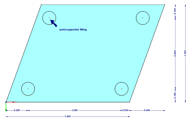
The transparency of the glass material should not be missing in any building. In addition to the typical application areas such as windows, this building material is increasingly being used for facades, canopies, or even as bracing of stairways. Of course, the planning architects often set a very high standard of transparency on fixation of the glass panes. This requires special glass fittings that couple the glass panes.
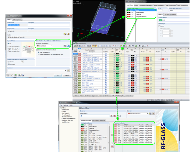
For the superposition or combination of loads, the German standard DIN 18008 refers to DIN 1055‑100. This also applies for the individual parameters of climatic loads to be transferred. In this case, it is possible to summarize the temperature change and meteorological pressure change in a single load and to define the local altitude change as a permanent load.
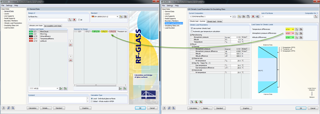
A new feature allows you to assign climatic loads to load cases when designing panes of insulating glass. Climatic loads are included in three categories here: temperature difference, atmospheric pressure difference, and altitude difference.
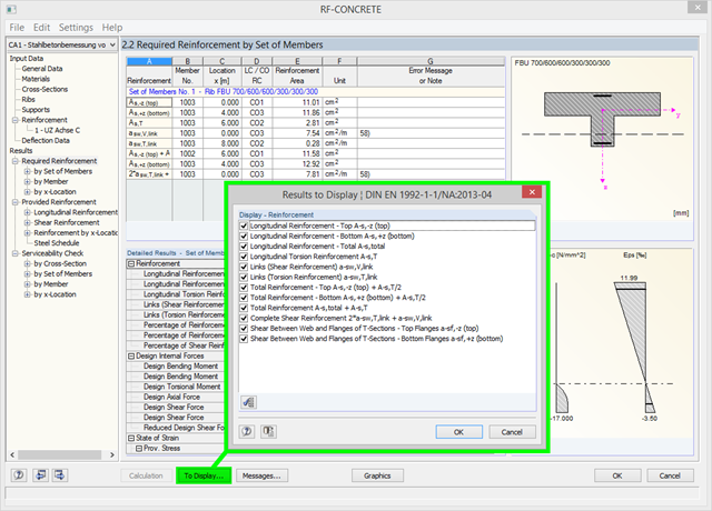
Using the [To Display…] button, you can specify the amount of reinforcement to be displayed in the results of the required reinforcement in Window 2.2 of RF‑CONCRETE and CONCRETE. In addition to the default setting, you can display the resulting reinforcement amount as (for example) the sum of the longitudinal and longitudinal torsion reinforcement, or the sum of the torsion and shear reinforcement. You can also reduce the number of preset results, of course.
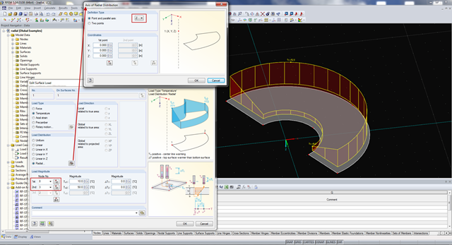
A new direction for temperature load is available in RFEM. Now, it is also possible to apply temperature loads with radial load distribution on a structure. The load is defined using an outer and an inner node, and an axis around which the radial load is applied.
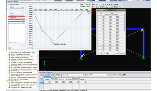
RF-/DYNAM Pro - Forced Vibrations provides the option of a time course monitor. During the evaluation process, you can compare several graphs directly in the program. In addition, you can transfer the figures to the printout report or export them directly to Excel as a value table.
Extensive calculations may result in vast amounts of data. Of course, current hard drives and SSDs are measured in terabytes. Therefore, you expect this to be no problem for current computing technology. This is true, in fact, but as often happens, the devil is in the details.