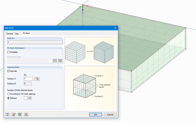
The stiffness of gas given by the ideal gas law pV = nRT can be considered in the nonlinear dynamic analysis.
The calculation of gas is available for accelerograms and time diagrams for both the explicit analysis and the nonlinear implicit Newmark analysis. To determine the gas behavior correctly, at least two FE layers for gas solids should be defined.
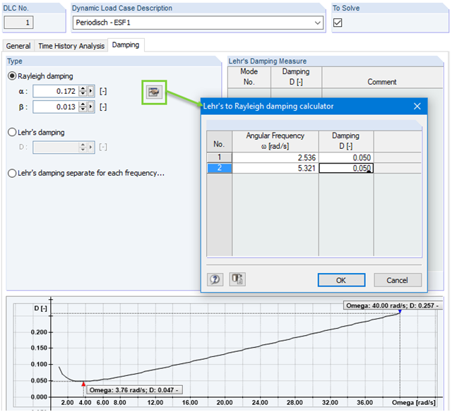
Calculation with consideration of a damping ratio (or Lehr's damping) is not possible in the direct time step integrations. Instead, the Rayleigh damping coefficients must be specified by the user.
In technical literature, the given damping ratio for specific construction forms is, in many cases, only a rough approximation of the real damping ratios. In RF-/DYNAM Pro - Forced Vibrations, it is possible to use the value of the damping ratio to determine the Rayleigh damping. This may occur at one or two natural angular frequencies defined by the user.
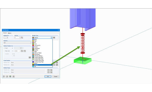
The member type 'Dashpot' can be used for time history analyzes in RFEM/RSTAB with the add-on modules RF-/DYNAM Pro - Forced Vibrations and RF-/DYNAM Pro - Nonlinear Time History. This linear viscous damping element considers forces dependent on velocity.
With regard to viscoelasticity, the member type 'Dashpot' is similar to the Kelvin-Voigt model, which consists of the damping element and an elastic spring (both connected in parallel).

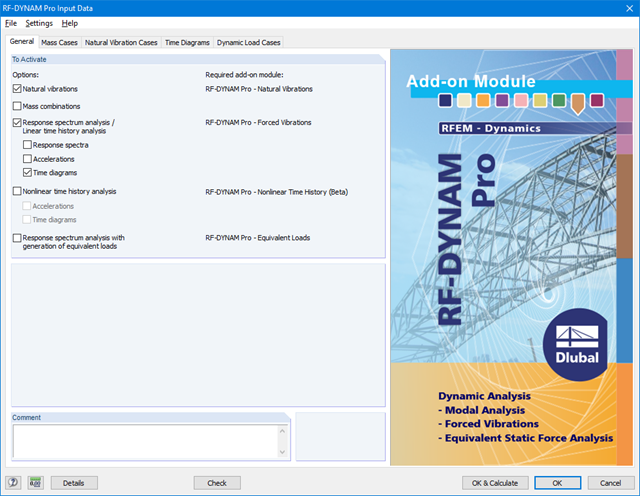
- Response spectra of numerous standards (ASCE 7-16, NBC 2015, etc.)
- User-defined response spectra or those generated from accelerograms
- Direction-relative response spectrum approach
- Manual or automatic selection of the relevant mode shapes of response spectra (5% rule of EC 8 applicable)
- Result combinations by modal superimposition (SRSS or CQC rule) and by direction superimposition (SRSS or 100% / 30% rule)
Due to the integration of RF‑/DYNAM Pro in RFEM / RSTAB, you can incorporate numeric and graphic results from RF‑/DYNAM Pro – Forced Vibrations in the global printout report. Also, all RFEM options are available for a graphical visualization.
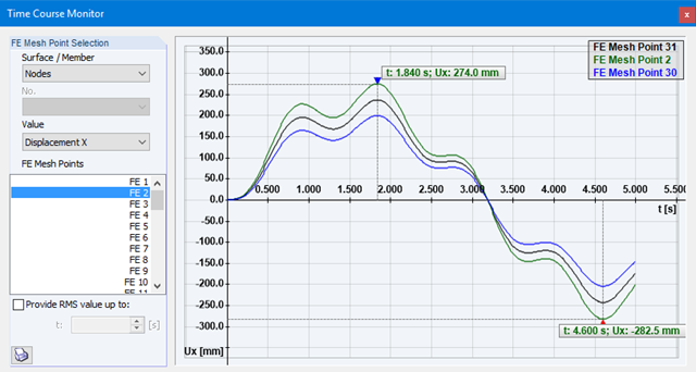
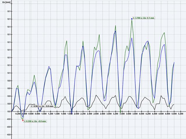
The results of the time history analysis are displayed in a time course monitor. All results are displayed as a function of time. You can export the numeric values to MS Excel.
In the case of a time history analysis, you can export results of the individual time steps or filter most unfavourable results of all time steps.
The response spectrum analysis generates result combinations. Internally, the modal contributions and the directional components of earthquake actions are combined.
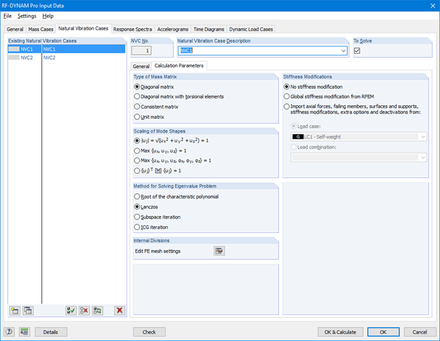
The time history analysis is performed with the modal analysis or the linear implicit Newmark analysis. The time history analysis in this add‑on module is restricted to linear systems. Although the modal analysis represents a fast algorithm, it is necessary to use a certain number of eigenvalues to ensure the required accuracy of results.
The implicit Newmark analysis is a very precise method, independent of the number of eigenvalues used, but requires sufficient small time steps for calculation. For the response spectra analysis, equivalent static loads are calculated internally. A linear static analysis is performed subsequently.
It is necessary to enter the required response spectra, accelerations, or time diagrams. Dynamic load cases define the location and direction of response spectra effects as well as acceleration time, or force-time excitations.
Timing diagrams are combined with static load cases, which provides great flexibility. For the time history analysis, you can import the initial deformation from any load case or load combination.
- Combination of user-defined time diagrams with load cases or load combinations (nodal, member, and surface loads, as well as free and generated loads, can be combined with time-variable functions)
- Combination of several independent excitation functions
- Extensive library of seismic events (accelerograms)
- Linear implicit Newmark analysis or modal analysis in time history
- Structural damping using Rayleigh damping coefficients or Lehr's damping
- Direct import of initial deformations from a load case or combination
- Graphical display of results in a time history diagram
- Export of results in user-defined time steps or as an envelope