
In RFEM and RSTAB, you can visualize the flow field quantities of pressure, velocity, turbulence kinetic energy, and turbulence dissipation rate for the wind simulation.
The clipping planes are aligned with the respective wind direction.

Are you looking for a formula relevant for your structural design? Just ask our AI chatbot Mia!
Mia shows you the right formula, with explanations, if necessary.

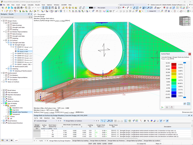
The building model is calculated in two phases:
- Global 3D calculation of the global model, where the slabs are modeled as a rigid plane (diaphragm) or as a bending plate
- Local 2D calculation of the individual floors
After the calculation, the results of the columns and walls from the 3D calculation and the results of the slabs from the 2D calculation are combined in a single model. This means that there is no need to switch between the 3D model and the individual 2D models of the slabs. The user only works with one model, saves valuable time, and avoids possible errors in the manual data exchange between the 3D model and the individual 2D ceiling models.
The vertical surfaces in the model can be divided into shear walls and opening lintels. The program automatically generates internal result members from these wall objects, so they can be designed as members according to any standard in the Concrete Design add-on.
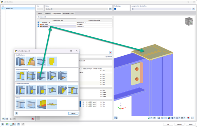
You can now insert a cap plate in steel joints with only a few clicks. You can enter the data using the known definition types "Offsets" or "Dimensions and Position". By specifying a reference member and the cutting plane, it is also possible to omit the Member Section component.
This component allows you to easily model cap plates on column ends, for example.
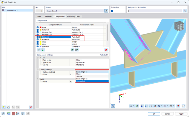
You can use the "Plate Cut" component to cut plates (for example, gusset plates, fin plates, and so on). There are various cutting methods available:
- Plane: The cut is performed on the closest surface to the reference plate.
- Surface: Only the intersecting parts of plates are cut.
- Bounding Box: The outermost dimension consisting of width and height is cut out of the plate as a rectangle.
- Convex Envelope: The outer hull of the cross-section is used for the plate cut. If there are fillets at the corner nodes of the cross-section, the cut is adapted to them.
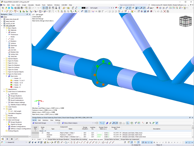
The Steel Joints add-on provides you with the option to connect circular hollow sections using welds.
It is possible to connect the circular sections to each other or to planar structural components. The fillets of standard and thin-walled sections can also be connected with a weld.
Go to Explanatory Video
Several modeling tools are available for elements in building models:
- Vertical line
- Column
- Wall
- Beam
- Rectangular floor
- Polygonal floor
- Rectangular floor opening
- Polygonal floor opening
This feature allows you to define the element on the ground plane (for example, with a background layer) with the associated multiple element creation in space.

Using the "Load Transfer Only" story type, you can consider slabs without stiffness effect in and out of the plane in the Building Model add-on. This element type collects the loads on the slab and transfers them to the supporting elements of a 3D model. Thus, you can simulate secondary components, such as grillage and similar load distribution elements, without any further effect in the 3D model.
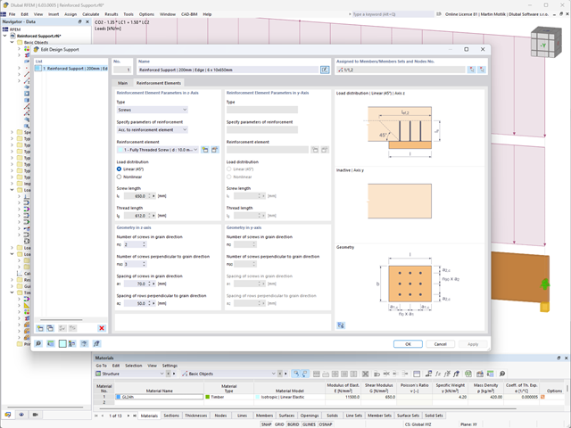
Did you know? In the Design Supports, you can now define fully threaded screws as transversal compression stiffening elements for the "Compression Perpendicular to Grain" design. In this case, the pressing-in and buckling of the bolts is analyzed.
Moreover, the design shear resistance is checked in the plane of the screw tip. The angle of dispersal can be considered as linear under 45° or nonlinear (according to Bejtka, I. (2005). Verstärkung von Bauteilen aus holz mit vollgewindeschrauben. KIT Scientific Publishing.).
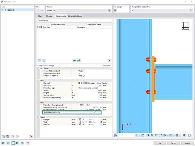
To determine the shear resistance of bolts, you can use the Steel Joints add-on to specify whether there is a shaft or a thread in the shear plane.
Go to Explanatory Video.png?mw=640&hash=55038d2a1591f62179796666cb9b2fede0274e19)
A graphical and tabular output of the results for deformations, stresses, and strains helps you when determining the soil solids. To achieve this, use the special filter criteria for targeted selection of results.
The program doesn't leave you alone with the results. If you want to graphically evaluate the results in the soil solids, you can use the guide objects. For example, you can define clipping planes. This allows you to view the corresponding results in any plane of the soil solid.
And not just that. The utilization of result sections and clipping boxes facilitates the precise graphical analysis of the soil solid.
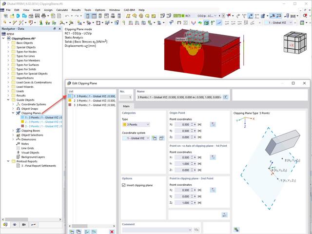
This feature also contributes to the clearly-arranged display of your results. Clipping planes are intersecting planes that you can place freely throughout the model. The zone in front of or behind the plane is consequently hidden in the display. This way, you can clearly and simply show the results in an intersection or a solid, for example.

As you've already learned, the results of a Modal Analysis load case are displayed in the program after a successful calculation. You can thus immediately see the first mode shape graphically or as an animation. You can also easily adjust the representation of the mode shape standardization. Do that directly in the Results navigator, where you have one of four options for the visualization of the mode shapes available for the selection:
- Scaling the value of the mode shape vector uj to 1 (considers the translation components only)
- Selecting the maximum translational component of the eigenvector and setting it to 1
- Considering the entire eigenvector (including the rotation components), selecting the maximum, and setting it to 1
- Setting the modal mass mi for each mode shape to 1 kg
You can find a detailed explanation of the mode shape standardization in the OnlineManual here.
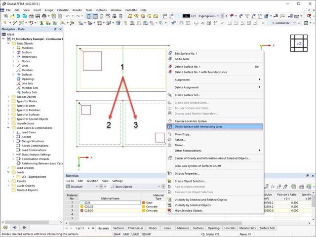
Planar surfaces can be divided by intersecting lines. The division can be done manually as follows:
- Select a surface with intersecting lines
- Use the "Divide Surface with Intersecting Lines" function
.png?mw=640&hash=342149908caead326e60e26a2b5d05f7f46825cb)
Are you familiar with the Tsai-Wu material model? It combines plastic and orthotropic properties, which allows for special modeling of materials with anisotropic characteristics, such as fiber-reinforced plastics or timber.
If the material is plastified, the stresses remain constant. The redistribution is carried out according to the stiffnesses available in the individual directions. The elastic area corresponds to the Orthotropic | Linear Elastic (Solids) material model. For the plastic area, the yielding according to Tsai-Wu applies:
All strengths are defined positively. You can imagine the stress criterion as an elliptical surface within a six-dimensional space of stresses. If one of the three stress components is applied as a constant value, the surface can be projected onto a three-dimensional stress space.
If the value for fy(σ), according to the Tsai-Wu equation, plane stress condition, is smaller than 1, the stresses are in the elastic zone. The plastic area is reached as soon as fy (σ) = 1; values greater than 1 are not allowed. The model behavior is ideal-plastic, which means there is no stiffening.

Did you know? In contrast to other material models, the stress-strain diagram for this material model is not antimetric to the origin. You can use this material model to simulate the behavior of steel fiber-reinforced concrete, for example. Find detailed information about modeling steel fiber-reinforced concrete in the technical article about Determining the material properties of steel-fiber-reinforced concrete.
In this material model, the isotropic stiffness is reduced with a scalar damage parameter. This damage parameter is determined from the stress curve defined in the Diagram. The direction of the principal stresses is not taken into account. Rather, the damage occurs in the direction of the equivalent strain, which also covers the third direction perpendicular to the plane. The tension and compression area of the stress tensor is treated separately. In this case, different damage parameters apply.
The "Reference element size" controls how the strain in the crack area is scaled to the length of the element. With the default value zero, no scaling is performed. Thus, the material behavior of the steel fiber concrete is modeled realistically.
Find more information about the theoretical background of the "Isotropic Damage" material model in the technical article describing the Nonlinear Material Model Damage.

- Numerous predefined components for easy input of typical connection situations (for example, end plates, angles, web plates)
- Universally applicable basic components (plates, welds, bolts, auxiliary planes) for the input of complex connection situations
- Graphical display of the connection geometry that is updated in parallel with the input
- The steel connection template included in the add-on allows you to select different connection types and apply them to your model
- The template provides connections from three categories: Rigid, Pinned, Truss
- Automatic adjustment of the connection geometry, even during subsequent editing of the structural components, due to the relative arrangement of the components to each other

Did you know that you can also display the moment-axial force interaction diagrams (M‑N diagrams) graphically? This allows you to display the cross-section resistance in the case of an interaction of a bending moment and an axial force. In addition to the interaction diagrams related to the cross-section axes (My‑N diagram and Mz‑N diagram), you can also generate an individual moment vector to create an Mres‑N interaction diagram. You can display the section plane of the M‑N diagrams in the 3D interaction diagram. The program displays the corresponding value pairs of the ultimate limit state in a table. The table is dynamically linked to the diagram so that the selected limit point is also displayed in the diagram.

Do you want to determine the biaxial bending resistance of a reinforced concrete cross-section? For this, you have to activate a moment-moment interaction diagram (My-Mz diagram) first. This My-Mz diagram represents a horizontal section through the three-dimensional diagram for the specified axial force N. Due to the coupling to the 3D interaction diagram, you can also visualize the section plane there.

You can be sure that costs are an important factor in the structural planning of any project. It is also essential to adhere to the provisions on emissions estimation. The two-part add-on Optimization & Costs/CO2 Emission Estimation makes it easier for you to find your way through the jungle of standards and options. It uses the artificial intelligence technology (AI) of the particle swarm optimization (PSO) to find the right parameters for parameterized models and blocks that guarantee the compliance with the usual optimization criteria. This add-on also estimates the model costs or CO2 emissions by specifying unit costs or emissions per material definition for the structural model. With this add-on, you are on the safe side.
More About Optimization & Costs / CO2 Emission Estimation
- Calculation of stationary incompressible turbulent wind flow using the SimpleFOAM solver from the OpenFOAM® software package
- Numerical scheme according to the first and second order
- Turbulence models RAS k-ω and RAS k-ε
- Consideration of surface roughness depending on model zones
- Model design via VTP, STL, OBJ, and IFC files
- Operation via bidirectional interface of RFEM or RSTAB for importing model geometries with standard-based wind loads and exporting wind load cases with probe-based printout report tables
- Intuitive model changes via drag & drop and graphical adjustment assistance
- Generation of a shrink-wrap mesh envelope around the model geometry
- Consideration of environmental objects (buildings, terrain, and so on)
- Height-dependent description of the wind load (wind speed and turbulence intensity)
- Automatic meshing depending on a selected depth of detail
- Consideration of layer meshes near the model surfaces
- Parallelized calculation with optimal utilization of all processor cores of a computer
- Graphical output of the surface results on the model surfaces (surface pressure, Cp coefficients)
- Graphical output of the flow field and vector results (pressure field, velocity field, turbulence – k-ω field, and turbulence – k-ε field, velocity vectors) on Clipper/Slicer planes
- Display of 3D wind flow via animated streamline graphics
- Definition of point and line probes
- Multilingual user interface (German, English, Czech, Spanish, French, Italian, Polish, Portuguese, Russian, and Chinese)
- Calculations of several models in one batch process
- Generator for creating rotated models to simulate different wind directions
- Optional interruption and continuation of the calculation
- Individual color panel per result graphic
- Display of diagrams with separate output of results on both sides of a surface
- Output of the dimensionless wall distance y+ in the mesh inspector details for the simplified model mesh
- Determination of the shear stress on the model surface from the flow around the model
- Calculation with an alternative convergence criterion (you can select between the residual types pressure or flow resistance in the simulation parameters)
By solving the numerical flow problem, you can obtain the following results on and around the model:
- Pressure on structure surface
- Coefficient Cp distribution on the structure surfaces
- Pressure field about the structure geometry
- Velocity field about the structure geometry
- Turbulence k-ω field about the structure geometry
- Turbulence k-ε field about the structure geometry
- Velocity vectors about the structure geometry
- Streamlines about the structure geometry
- Forces on member-shaped structures that were originally generated from member elements
- Convergence diagram
- Direction and size of the flow resistance of the defined structures
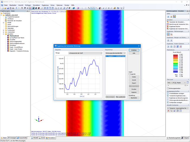
Despite this amount of information, RWIND 2 remains clearly arranged, as is typical for the Dlubal programs. You can specify freely definable zones for a graphic evaluation. Voluminously displayed flow results about the structure geometry are often confusing – you know the problem for sure. That's why RWIND Basic provides freely movable section planes for the separate display of the "solid results" in a plane. For the 3D branched streamline result, you have an option to select between a static and an animated display in the form of moving line segments or particles. This option helps you to represent the wind flow as a dynamic effect.
You can export all results as a picture or, especially for the animated results, as a video.
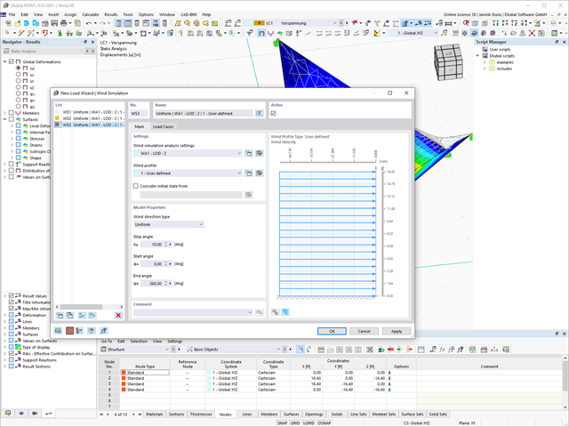
Discover the new features in RFEM and RSTAB for the determination of wind loads using RWIND:
- Useful load wizards for generating wind load cases with different flow fields in different wind directions
- Wind load cases with freely assignable analysis settings including a user-defined specification of the wind tunnel size and wind profile
- Comprehensive display of the wind tunnel with input wind profile and turbulence intensity profile
- Visualization and use of the RWIND simulation results
- Global definition of a terrain (horizontal planes, inclined plane, table)
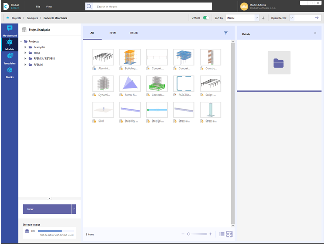
The Dlubal Center ensures that your planning goes quickly and efficiently. Among other things, your projects and model files are managed here in a central location. Detailed information and graphics make it easier for you to assign all models and thus enable uncomplicated, clear processing of the project. Furthermore, your customer data including the licensed programs and add-ons is organized in the Dlubal Center.
More About Dlubal Center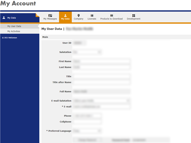
Dlubal Software supports its customers with their construction planning worldwide. The modern online licensing system allows licenses of RFEM, RSTAB, and other programs to be distributed all over the world and assigned to the respective users via the Dlubal Account.
Go to Explanatory Video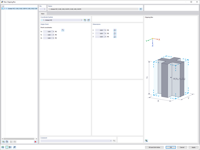
Keep track of what's really relevant to your project. In addition to the clipping plane, you can now define a clipping box. This allows you to hide the irrelevant objects around a focal point.

Do you know exactly how the form-finding is performed? First, the form-finding process of the load cases with the load case category "Prestress" shifts the initial mesh geometry to an optimally balanced position by means of iterative calculation loops. For this task, the program uses the Updated Reference Strategy (URS) method by Prof. Bletzinger and Prof. Ramm. This technology is characterized by equilibrium shapes that, after the calculation, comply almost exactly with the initially specified form-finding boundary conditions (sag, force, and prestress).
In addition to the pure description of the expected forces or sags on the elements to be formed, the integral approach of the URS also enables a consideration of regular forces. In the overall process, this allows, for example, for a description of the self-weight or a pneumatic pressure by means of corresponding element loads.
All these options give the calculation kernel the potential to calculate anticlastic and synclastic forms that are in an equilibrium of forces for planar or rotationally symmetric geometries. In order to be able to realistically implement both types individually or together in one environment, the calculation provide you with two ways to describe the form-finding force vectors:
- Tension method - description of the form-finding force vectors in space for planar geometries
- Projection method - description of the form-finding force vectors on a projection plane with fixation of the horizontal position for conical geometries
_(1).png?mw=640&hash=415f7bbaf70e41679bb0106e1cf91eaa8c493ec9)
- Automatic generation of FE analysis models: The add-on automatically creates a finite element model (FE) of the steel connection in the background.
- Consideration of all internal forces: The calculation and design checks include all internal forces (N, Vy, Vz, My, Mz, MT) and are not limited to planar loading.
- Automatic load transfer: All load combinations are automatically transferred to the FE analysis model of the connection. The loads are transferred directly from RFEM, so manual data input is not necessary.
- Efficient modeling: The add-on saves you time when modeling complex connection situations. You can also save the created FE analysis model and use it further for your own detailed analyses.
- Extensible library: An extensive and extensible library with predefined steel connection templates is available.
- Wide applicability: The add-on is suitable for connections of any type and shape, compatible with almost all rolled, welded, built-up, and thin-walled cross-sections.

- Selection of nodes in the RFEM model, automatic recognition and assignment of the members connected to the node
- Many predefined components available for easy input of typical connection situations (for example, end plates, cleats, fin plates)
- Universally applicable basic components (plates, welds, auxiliary planes) for entering complex connection situations
- No manual editing of the FE model required by the user, the essential calculation settings can be changed via the configuration settings
- Automatic adaptation of the connection geometry, even if the members are subsequently edited, due to the relative relation of the components to each other
- Parallel to the input, a plausibility check is carried out by the program to quickly detect missing input or collisions, for example
- Graphical display of the connection geometry that is updated in parallel with the input
- Automatic import of internal forces from RFEM/RSTAB
- Optional consideration of creep
- Automatic determination of planned and unintentional eccentricity from the second-order analysis in addition to the existing eccentricity
- Determination of internal forces according to the linear static analysis and the second-order analysis
- Analysis of governing design locations along the column due to existing loading
- Output of the required longitudinal and stirrup reinforcement
- Summary of design ratios, including all design details