
In the Modal Analysis add-on, you have the option to automatically increase the sought eigenvalues until reaching a defined effective modal mass factor. All translational directions activated as masses for the modal analysis are taken into account.
Thus, it is possible to easily calculate the required 90% of the effective modal mass for the response spectrum method.
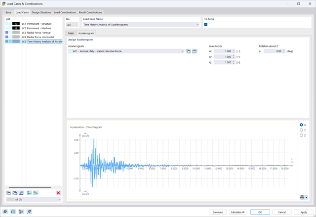
The Time History Analysis add-on provides you with accelerograms for the calculation. This extension allows for dynamic structural analysis of the acceleration-time diagrams.
There is an extensive library of earthquake records available for you, but you can also enter or import your own diagrams. The time history analysis is performed using the modal analysis or the linear implicit Newmark analysis.

The modal relevance factor (MRF) can help you to assess to which extent specific elements participate in a specific mode shape. The calculation is based on the relative elastic deformation energy of each individual member.
The MRF can be used to distinguish between local and global mode shapes. If multiple individual members show significant MRF (for example, > 20%), the instability of the entire structure or a substructure is very likely. On the other hand, if the sum of all MRFs for an eigenmode is around 100%, a local stability phenomenon (for example, buckling of a single bar) can be expected.
Furthermore, the MRF can be used to determine critical loads and equivalent buckling lengths of certain members (for example, for stability design). Mode shapes for which a specific member has small MRF values (for example, < 20%) can be neglected in this context.
The MRF is displayed by mode shape in the result table under Stability Analysis → Results by Members → Effective Lengths and Critical Loads.
- Analysis of time diagrams and accelerograms (acceleration-time diagrams exciting the supports of a structure)
- Combination of user-defined time diagrams with nodal, member, and surface loads, as well as free and generated loads
- Combination of several independent excitation functions
- Linear implicit Newmark analysis or modal analysis in time history
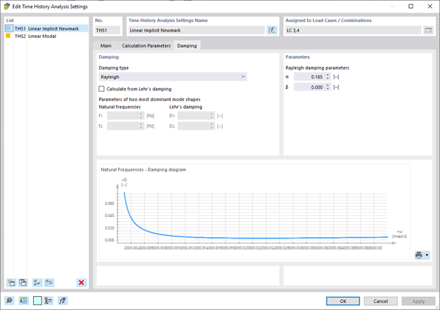
- Structural damping using Raleigh damping coefficients or Lehr's damping value
- Graphical display of results in calculation diagrams
- Result display in individual time steps or as an envelope during the entire time period
- Extensive library of seismic events (accelerograms)
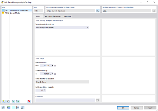
The time history analysis is performed with the modal analysis or the linear implicit Newmark analysis. The time history analysis in this add-on is limited to linear structural systems. Although the modal analysis represents a fast algorithm, it is necessary to use a certain number of eigenvalues to ensure the required accuracy of results.
The implicit Newmark analysis is a very precise method, independent of the number of eigenvalues used, but requires sufficient small time steps for the calculation.

Have you already discovered the tabular and graphical output of masses in mesh points? That's right, this is also part of the modal analysis results in RFEM 6. This way, you can check the imported masses that depend on various settings of the modal analysis. They can be displayed in the Masses in Mesh Points tab of the Results table. The table provides you with an overview of the following results: Mass - Translational Direction (mX, mY, mZ), Mass - Rotational Direction (mφX, mφY, mφZ), and the Sum of Masses. Would it be best for you to have a graphical evaluation as quickly as possible? Then you can also graphically display the masses in mesh points.

As you've already learned, the results of a Modal Analysis load case are displayed in the program after a successful calculation. You can thus immediately see the first mode shape graphically or as an animation. You can also easily adjust the representation of the mode shape standardization. Do that directly in the Results navigator, where you have one of four options for the visualization of the mode shapes available for the selection:
- Scaling the value of the mode shape vector uj to 1 (considers the translation components only)
- Selecting the maximum translational component of the eigenvector and setting it to 1
- Considering the entire eigenvector (including the rotation components), selecting the maximum, and setting it to 1
- Setting the modal mass mi for each mode shape to 1 kg
You can find a detailed explanation of the mode shape standardization in the OnlineManual here.

Do you want to consider other loads as masses in addition to the static loads? The program allows that for nodal, member, line and surface loads. For this, you need to select the Mass load type when defining the load of interest. Define a mass or mass components in the X, Y, and Z directions for such loads. For nodal masses, you have an additional option to also specify moments of inertia X, Y, and Z in order to model more complex mass points.

It is often necessary to neglect masses. This is particularly the case when you want to use the output of the modal analysis for the seismic analysis. For this, 90% of the effective modal mass in each direction is required for the calculation. So you can neglect the mass in all fixed nodal and line supports. The program automatically deactivates the associated masses for you.
You can also manually select the objects whose masses are to be neglected for the modal analysis. We have shown the latter in the image for a better view. A user-defined selection is made the and the objects with their associated mass components are selected to neglect the masses.

When defining the input data for the modal analysis load case, you can consider a load case whose stiffnesses represent the initial position for the modal analysis. How do you do that? As shown in the image, select the "Consider initial state from" option. Now, open the "Initial State Settings" dialog box and define the type Stiffness as the initial state. In this load case, as of which is the initial state taken into account, you can consider the stiffness of the structural system when the tension members fail. The purpose of all of this: The stiffness from this load case is considered in the modal analysis. Thus, you obtain a clearly flexible system.

You can already see it in the image: Imperfections can also be taken into account when defining a modal analysis load case. The imperfection types that you can use in the modal analysis are notional loads from load case, initial sway via table, static deformation, buckling mode, dynamic mode shape, and group of imperfection cases.

Did you know? You can easily define structural modifications in load cases of the Modal Analysis type. This allows you, for example, to individually adjust the stiffnesses of materials, cross-sections, members, surfaces, hinges, and supports. You can also modify stiffnesses for some design add-ons. Once you select the objects, their stiffness properties are adapted to the object type. In this way, you can define them in separate tabs.
Do you want to analyze the failure of an object (for example, a column) in the modal analysis? This is also possible without any problems. Simply switch to the Structure Modification window and deactivate the relevant objects.

Is your goal to determine the number of mode shapes? The program offers you two methods for this. On the one hand, you can manually define the number of the smallest mode shapes to be calculated. In this case, the number of available mode shapes depends on the degrees of freedom (that is, the number of free mass points multiplied by the number of directions in which the masses act). However, it is limited to 9999. On the other hand, you can set the maximum natural frequency the way that the program determined the mode shapes automatically until reaching the natural frequency set.

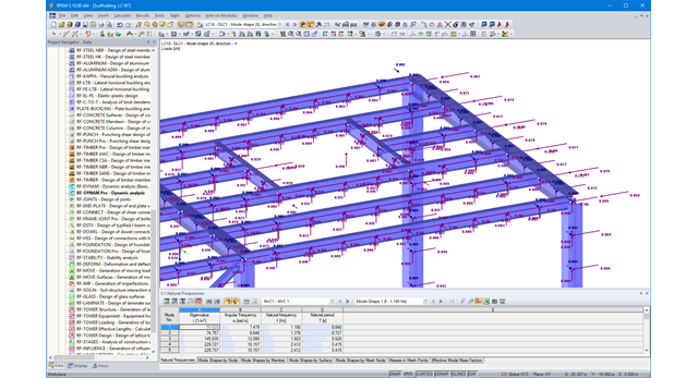
Is the calculation finished? The results of the modal analysis are then available both graphically and in tables. Display the result tables for the load case or the load cases of the modal analysis. Thus, you can see the eigenvalues, angular frequencies, natural frequencies, and natural periods of the structure at first glance. The effective modal masses, modal mass factors, and participation factors are also clearly displayed.

You have several options available to define masses for a modal analysis. While the masses due to self-weight are considered automatically, you can consider the loads and masses directly in a load case of the modal analysis type. Do you need more options? Select whether to consider full loads as masses, load components in the global Z-direction, or only the load components in the direction of gravity.
The program offers you an additional or alternative option for importing masses: A manual definition of load combinations as of which are the masses considered in the modal analysis. Have you selected a design standard? You can then create a design situation with the Seismic Mass combination type. Thus, the program automatically calculates a mass situation for the modal analysis according to the preferred design standard. In other words: The program creates a load combination on the basis of the preset combination coefficients for the selected standard. This contains the masses used for the modal analysis.
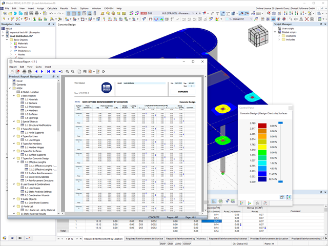
Discover the fundamentally revised and optimized printout report. It offers you the following innovations, among other things:
- Quick creation due to non-modal printout report environment (parallel work in program and report possible)
- Interactive modification of chapters as well as creation of new user-defined chapters
- Import of PDFs, formulas, 3D graphics, and so on
- Output of the design check formulas used in the design (including a reference to the used equation from the standard)
- Modern printout report design

Compared to the RF‑/DYNAM Pro - Natural Vibrations add-on module (RFEM 5 / RSTAB 8), the following new features have been added to the Modal Analysis add-on for RFEM 6 / RSTAB 9:
- Preset combination coefficients for various standards (EC 8, ASCE, and so on)
- Optional neglect of masses (for example, mass of foundations)
- Methods for determining the number of mode shapes (user-defined, automatic - to reach effective modal mass factors, automatic - to reach the maximum natural frequency)
- Output of modal masses, effective modal masses, modal mass factors, and participation factors
- Masses in mesh points displayed in tables and graphics
- Various scaling options for mode shapes in the Result navigator

Compared to the RF‑/STEEL add-on module (RFEM 5 / RSTAB 8), the following new features have been added to the Stress-Strain Analysis add-on for RFEM 6 / RSTAB 9:
- Treatment of members, surfaces, solids, welds (line welded joints between two and three surfaces with subsequent stress design)
- Output of stresses, stress ratios, stress ranges, and strains
- Limit stress depending on the assigned material or a user-defined input
- Individual specification of the results to be calculated through freely assignable setting types
- Non-modal result details with prepared formula display and additional result display on the cross-section level of members
- Output of the design check formulas used

The load cases of the type Response Spectrum Analysis contain the generated equivalent loads. First, the modal contributions have to be superimposed with the SRSS or CQC rule. In this case, you can use the signed results based on the dominant mode shape.
Afterwards, the directional components of earthquake actions are combined with the SRSS or the 100% / 30% rule.

- Automatic consideration of masses from self-weight
- Direct import of masses from load cases or load combinations
- Optional definition of additional masses (nodal, linear, or surface masses, as well as inertia masses) directly in the load cases
- Optional neglect of masses (for example, mass of foundations)
- Combination of masses in different load cases and load combinations
- Preset combination coefficients for various standards (EC 8, SIA 261, ASCE 7,...)
- Optional import of initial states (for example, to consider prestress and imperfection)
- Structure Modification
- Consideration of failed supports or members/surfaces/solids
- Definition of several modal analyses (for example, to analyze different masses or stiffness modifications)
- Selection of mass matrix type (diagonal matrix, consistent matrix, unit matrix), including user-defined specification of translational and rotational degrees of freedom
- Methods for determining the number of mode shapes (user-defined, automatic - to reach effective modal mass factors, automatic - to reach the maximum natural frequency - only available in RSTAB)
- Determination of mode shapes and masses in nodes or FE mesh points
- Results of eigenvalue, angular frequency, natural frequency, and period
- Output of modal masses, effective modal masses, modal mass factors, and participation factors
- Masses in mesh points displayed in tables and graphics
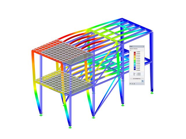
- Visualization and animation of mode shapes
- Various scaling options for mode shapes
- Documentation of numerical and graphical results in printout report

In the modal analysis settings, you have to enter all data that are necessary for the determination of the natural frequencies. These are, for example, mass shapes and eigenvalue solvers.
The Modal Analysis add-on determines the lowest eigenvalues of the structure. Either you adjust the number of eigenvalues or let them determined automatically. Thus, you should reach either effective modal mass factors or maximum natural frequencies. Masses are imported directly from load cases and load combinations. In this case, you have the option to consider the total mass, load components in the global Z-direction, or only the load component in the direction of gravity.
You can manually define additional masses at nodes, lines, members, or surfaces. Furthermore, you can influence the stiffness matrix by importing axial forces or stiffness modifications of a load case or load combination.

In RFEM, you can use these three powerful eigenvalue solvers:
- Root of Characteristic Polynomial
- Method by Lanczos
- Subspace Iteration
RSTAB, on the other hand, provides you with these two eigenvalue solvers:
- Subspace Iteration
- Shifted inverse power method
The selection of the eigenvalue solver depends primarily on your model size.

As soon as the program has completed the calculation, the eigenvalues, natural frequencies and periods are listed. These result windows are integrated in the main program RFEM/RSTAB. You can find all mode shapes of the structure in tables and also have an option to display them graphically and to animate them.
All result tables and graphics are part of the RFEM/RSTAB printout report. In this way, you can ensure clearly arranged documentation. You can also export the tables to MS Excel.
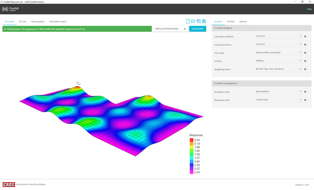
There is a known complexity in calculating footfall response on irregular floors or staircases of any type. Footfall Analysis uses the RFEM model and the modal analysis results of RF-DYNAM Pro - Natural Vibrations to predict the vibration levels at all locations on a floor. A rigorous analysis method is essential to enable an accurate investigation of the dynamic behavior of the floor.
The software incorporates the most up-to-date analysis procedures, allowing the user to select between the two most often used calculation methods available, namely the Concrete Centre Method (CCIP-016) and the Steel Construction Institute Method (P354).
- Response spectra in accordance with different standards
- The following standards are implemented:
-
 EN 1998-1:2010 + A1:2013 (European Union)
 -
 DIN 4149:1981-04 (Germany)
 -
DIN 4149:2005-04 (Germany)
-
 IBC 2000 (USA)
 -
IBC 2009-ASCE/SEI 7-05 (USA)
-
IBC 2012/15 - ASCE/SEI 7-10 (USA)
-
IBC 2018 - ASCE/SEI 7-16 (USA)
-
 ÖNORM B 4015:2007-02 (Austria)
 -
 NTC 2018 (Italy)
 -
 NCSE-02 (Spain)
 -
 SIA 261/1:2003 (Switzerland)
 -
SIA 261/1:2014 (Switzerland)
-
SIA 261/1: 2020 (Switzerland)
-
 O.G. 23089 + OG 23390 (Turkey)
 -
 SANS 10160-4 2010 (South Africa)
 -
 SBC 301:2007 (Saudi Arabia)
 -
 GB 50011 - 2001 (China)
 -
GB 50011 - 2010 (China)
-
 NBC 2015 (Canada)
 -
 DTR BC 2-48 (Algeria)
 -
DTR RPA99 (Algeria)
-
 CFE Sismo 08 (Mexico)
 -
 CIRSOC 103 (Argentina)
 -
 NSR - 10 (Colombia)
 -
 IS 1893:2002 (India)
 -
 AS1170.4 (Australia)
 -
 NCh 433 1996 (Chile)
-
- The following National Annexes according to EN 1998‑1 are available:
-
DIN EN 1998-1/NA:2011-01 (Germany)
-
ÖNORM EN 1991-1-1:2011-09 (Austria)
-
 NBN - ENV 1998-1-1: 2002 NAD-E/N/F (Belgium)
 -
 ČSN EN 1998-1/NA:2007 (Czech Republic)
 -
 NF EN 1998-1-1/NA:2014-09 (France)
 -
UNI-EN 1991-1-1/NA:2007 (Italy)
-
 NP EN 1998-1/NA:2009 (Portugal)
 -
 SR EN 1998-1/NA:2004 (Romania)
 -
 STN EN 1998-1/NA:2008 (Slovakia)
 -
 SIST EN 1998-1:2005/A101:2006 (Slovenia)
 -
 CYS EN 1998-1/NA:2004 (Cyprus)
 -
 NA to BS EN 1998-1:2004:2008 (United Kingdom)
 - NS-EN 1998-1:2004 + A1:2013/NA:2014 (Norway)
-
- User-defined response spectra
- Direction-relative response spectrum approach
- Relevant mode shapes for the response spectrum can be selected manually or automatically (5% rule from EC 8 can be applied)
- Generated equivalent static loads are exported to load cases, separately for each modal contribution and separately for each direction
- Result combinations by modal superposition (SRSS and CQC rule) and direction superposition (SRSS or 100% / 30% rule)
- Signed results based on the dominant eigenmode can be displayed
- Automatic consideration of masses from self-weight
- Direct import of masses from load cases or load combinations
- Optional definition of additional masses (nodal, linear, surface masses, as well as inertia masses)
- Combination of masses in different mass cases and mass combinations
- Preset combination coefficients according to EC 8
- Optional import of normal force distributions (in order to consider prestress, for example)
- Stiffness modification (for example, deactivated members or stiffnesses can be imported from RF-/CONCRETE)
- Consideration of failed supports or members
- Definition of several natural vibration cases (for example, to analyze different masses or stiffness modifications)
- Results of eigenvalue, angular frequency, natural frequency, and period
- Determination of mode shapes and masses in nodes or FE mesh points
- Results of modal masses, effective modal masses, and modal mass factors
- Visualization and animation of mode shapes
- Various scaling options for mode shapes
- Documentation of numerical and graphical results in the printout report

- Response spectra of numerous standards (ASCE 7-16, NBC 2015, etc.)
- User-defined response spectra or those generated from accelerograms
- Direction-relative response spectrum approach
- Manual or automatic selection of the relevant mode shapes of response spectra (5% rule of EC 8 applicable)
- Result combinations by modal superimposition (SRSS or CQC rule) and by direction superimposition (SRSS or 100% / 30% rule)
The equivalent load analysis calculation generates load cases and result combinations. The load cases include the generated equivalent loads, which are subsequently superimposed in result combinations. First, the modal contributions are superimposed with the SRSS or CQC rule. Signed results based on the dominant mode shape are possible.
Afterwards, the directional components of earthquake actions are combined with the SRSS or the 100% / 30% rule.
Due to the integration of RF‑/DYNAM Pro in RFEM / RSTAB, you can incorporate numeric and graphic results from RF‑/DYNAM Pro – Forced Vibrations in the global printout report. Also, all RFEM options are available for a graphical visualization.
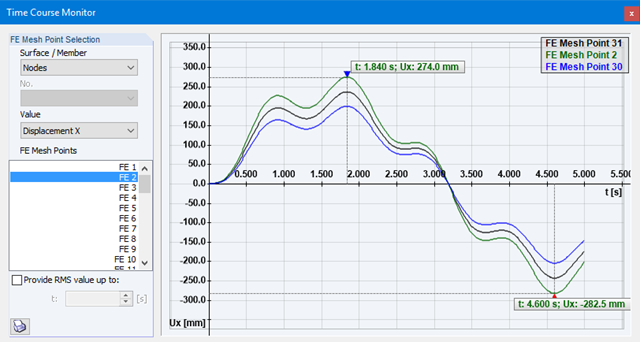
The results of the time history analysis are displayed in a time course monitor. All results are displayed as a function of time. You can export the numeric values to MS Excel.
In the case of a time history analysis, you can export results of the individual time steps or filter most unfavourable results of all time steps.
The response spectrum analysis generates result combinations. Internally, the modal contributions and the directional components of earthquake actions are combined.
The time history analysis is performed with the modal analysis or the linear implicit Newmark analysis. The time history analysis in this add‑on module is restricted to linear systems. Although the modal analysis represents a fast algorithm, it is necessary to use a certain number of eigenvalues to ensure the required accuracy of results.
The implicit Newmark analysis is a very precise method, independent of the number of eigenvalues used, but requires sufficient small time steps for calculation. For the response spectra analysis, equivalent static loads are calculated internally. A linear static analysis is performed subsequently.