Program RFEM 6 do analizy statyczno-wytrzymałościowej jest podstawą systemu modułowego. Program główny RFEM 6 służy do definiowania konstrukcji, materiałów i obciążeń płaskich i przestrzennych układów konstrukcyjnych składających się z płyt, ścian, powłok i prętów. Program umożliwia również tworzenie konstrukcji mieszanych oraz modelowanie elementów bryłowych i kontaktowych.
RSTAB 9 to wydajne oprogramowanie do obliczeń konstrukcji szkieletowych 3D, odzwierciedlające aktualny stan wiedzy i pomagające inżynierom sprostać wymaganiom współczesnej inżynierii lądowej.
Często zbyt długo zajmujesz się obliczaniem przekrojów? Oprogramowanie firmy Dlubal i program samodzielny RSECTION ułatwiają pracę, określając i przeprowadzając analizę naprężeń dla różnych przekrojów.
Czy zawsze wiesz, skąd wieje wiatr? Oczywiście od strony innowacji! RWIND 3 to program, który wykorzystuje cyfrowy tunel aerodynamiczny do numerycznej symulacji przepływu wiatru. Program symuluje przepływ wokół dowolnej geometrii budynku i określa obciążenia wiatrem na powierzchnie.
Szukasz narzędzia do przeglądu stref obciążenia śniegiem, wiatrem i trzęsieniem ziemi? Dobrze trafiłeś! Skorzystaj z narzędzia do geolokalizacji do szybkiego i skutecznego definiowania obciążenia śniegiem, prędkości wiatru, obciążenia trzęsieniem ziemi, zgodnie z Eurokodem i innymi międzynarodowymi normami.
Chcesz wypróbować możliwości programów Dlubal Software? To Twoja szansa! Dzięki 90-dniowej pełnej wersji, możesz w pełni przetestować wszystkie nasze programy.
Norma ASCE 7-22 oferuje kilka typów widm obliczeniowych. W tym FAQ chcielibyśmy skoncentrować się na następujących dwóch widmach obliczeniowych:
Widmo dwuokresowe jest normalnie zapisywane w programie. Jednak na podstawie danych dostępnych w normie można zaproponować tylko horyzontalne spektrum obliczeniowe/widmo MCER oraz modyfikację związaną z siłą i przemieszczeniem.
Dla wielookresowego spektrum obliczeniowego określane są dyskretne wartości liczbowe. W normie ASCE 7-22 podano, że wartości te można sprawdzić na stronie geobazy USGS Seismic Design Geodatabase. W obecnym stanie rozwoju istnieje możliwość utworzenia zdefiniowanego przez użytkownika spektrum odpowiedzi ze współczynnikiem g (w zależności od -6/000369 stała konwersji masy ), aby wykorzystać dane np. z ASCE 7 Hazard Tool [1].
Proszę postępować w następujący sposób:
Programy RFEM i RSTAB stosują inną odmianę metody modułu sprężystości podłoża. Eine Beziehung auf den Steifemodul ES ist nicht möglich.
In RFEM ist ein mehrparametrisches Bettungsmodell implementiert. Damit können realistische Setzungsberechnungen durchgeführt werden.
Ein Problem ist es jedoch, genaue Werte für die Parameter Cu,z, Cv,xz und Cv,yz zu finden. Hierbei unterstützt Sie das Add-On Geotechnische Analyse (für RFEM 6) bzw. das Zusatzmodul RF-SOILIN (für RFEM 5): Aus den Belastungen und den Daten des Baugrundgutachtens (Steifeziffer oder E-Modul und Querdehnzahl, Wichte, Schichtdicken) werden für jedes einzelne finite Element mit einem nichtlinearen Verfahren die Bettungsparameter berechnet. Diese Parameter sind lastabhängig und beeinflussen ihrerseits wieder das Verhalten des Bauwerks. Das Ergebnis dieses iterativen Prozesses sind realistische Setzungen und Schnittgrößen im Bauwerk.
Domyślnie aktywna jest opcja Płaszczyzna ścinania w gwincie, a do sprawdzenia ścinania w śrubie jest brana pod uwagę niższa wytrzymałość zgodna z wybraną normą obliczeniową.
W AISC nominalne wytrzymałości śrub na ścinanie są podane w tabeli J3.2. Na przykład, śruba z grupy A (na przykład A325) ma nominalną wytrzymałość na ścinanie równą 54 ksi (372 MPa), gdy gwint nie jest wykluczony z płaszczyzn ścinania. Aby użyć wyższej wytrzymałości, wynoszącej 68 ksi (469 MPa), można odznaczyć opcję, aby wykluczyć gwinty z płaszczyzn ścinania.
Za pomocą szablonu „Płyta-płyta” z biblioteki Komponenty (rysunek 01) można za pomocą blach czołowych w prosty sposób utworzyć połączenie nakładkowe.
W przypadku połączenia nakładkowego bez blach czołowych konfigurację można utworzyć ręcznie, dodając poszczególne komponenty (rysunek 02).
Konfiguracja obejmuje następujące komponenty. Każdy komponent można łatwo usunąć lub skopiować, klikając w niego prawym przyciskiem myszy.
Wymagane jest utworzenie niewielkiej przerwy przy użyciu funkcji „Pręt cięcia” i „Płaszczyzny pomocniczej”. Odstęp jest dzielony między dwa pręty (tzn. odstęp 1/16” jest stosowany jako przemieszczenie o 1/32” do każdego pręta).
Alternatywnie, przykładowy model „AISC Splice Connection” można pobrać i zapisać jako szablon zdefiniowany przez użytkownika (zdjęcie 03).
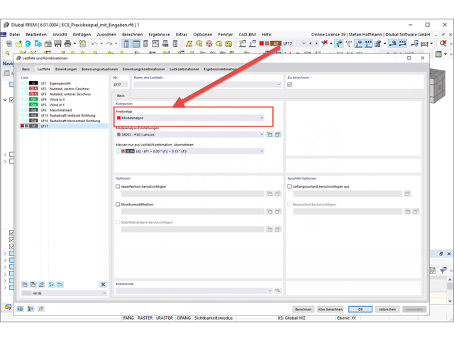
W przypadku obciążenia typu Analiza modalna można również zdefiniować zmiany konstrukcyjne. W ten sposób można uzyskać dostęp do modyfikacji sztywności poszczególnych obiektów, a w razie potrzeby również dezaktywować wybrane obiekty.
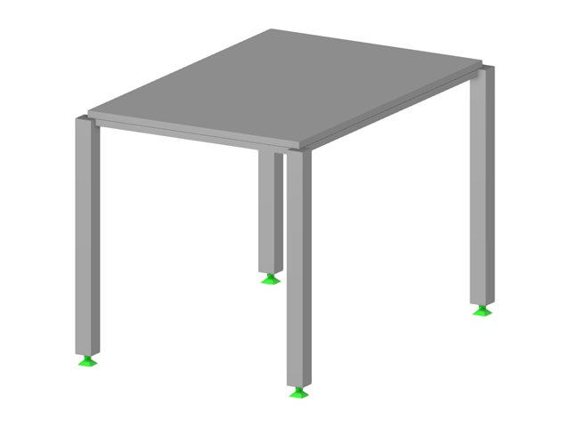
Aby wyświetlić kształty drgań własnych w analizie dynamicznej, należy utworzyć przypadek obciążenia typu Analiza modalna i określić w nim ustawienia dla analizy modalnej.
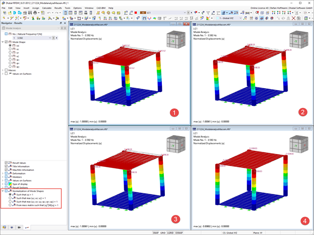
Po zakończeniu obliczeń można ocenić uzyskane wyniki w nawigatorze Wyniki. W tabeli można również znaleźć dalsze informacje.
Bezpośrednio w nawigatorze Wyniki można dostosować wyświetlanie normalizacji postaci drgań własnych. W przypadku zmiany ustawienia nie jest konieczne ponowne obliczanie.
W zależności od ustawienia największe przemieszczenie lub odkształcenie stanowi wartość odniesienia 1, do której skalowane są pozostałe wyniki.
Geometria brył gruntowych masywu gruntowego może być edytowana ręcznie, jeżeli w oknie wprowadzania danych zostanie ustawiony typ "Zbiór brył gruntowych".
Krok 1 (opcjonalnie) - Masyw gruntowy z próbek gruntu
Masyw można początkowo wygenerować z próbek gruntu, aby wykorzystać zalety wygenerowanych brył gruntowych z materiałami gruntowymi i interfejsami warstw, które wynikają z danych z badań podłoża gruntowego zawartych w próbkach gruntu.Można to zrobić w pierwszym kroku, jak pokazano na rysunku 1.
Krok 2 - Określ typ zbioru brył gruntowych
W drugim kroku typ gruntu stałego można zmienić z (1) wygenerowanego na podstawie próbek gruntu na (2) zbiór brył gruntu. Po potwierdzeniu tego kroku pojawiają się obliczone współrzędne masywu gruntowego. Rysunek 2 przedstawia ten krok w oknie dialogowym Masyw gruntowy.
Uwaga: Należy zauważyć, że ten krok usuwa status "wygenerowany", co skutkuje między innymi rozłączeniem połączenia z próbkami gleby w celu umożliwienia edycji.
Krok 3 - Edycja geometrii brył gruntowych
Bryły gruntowe można teraz edytować, a żądaną geometrię powierzchni terenu można wygenerować za pomocą wszystkich środków dostępnych i znanych w programie RFEM 6. Ten krok można zobaczyć na rysunku 3.
Poniższy rysunek przedstawia przykład geometrii masywu gruntowego utworzonego zgodnie z krokami od 1 do 3.
Aby przeprowadzić analizę trzęsienia ziemi, potrzebna jest analiza modalna, a następnie przypadek obciążenia typu Analiza spektrum odpowiedzi.
Po przeprowadzeniu analizy modalnej należy utworzyć nowy przypadek obciążenia. Tutaj znajdują się zwykłe ustawienia z poprzedniej generacji programu.
W zakładce Spektrum odpowiedzi można zdefiniować swoje spektrum odpowiedzi w zwykły sposób. Jeżeli chcesz użyć spektrum odpowiedzi zgodnie z normą, upewnij się, że w danych ogólnych normy II wybrano żądaną normę.
W zakładce Wybór trybów można wybrać kształty postaci i w razie potrzeby przefiltrować je.
Po obliczeniu przypadku obciążenia otrzymujemy wyniki.
W ustawieniach analizy modalnej można ustawić minimalne odkształcenie osiowe dla kabli i membran, aby zastosować początkowe naprężenie wstępne dla obiektów, a tym samym poprawić zbieżność obliczeń. Wstępne naprężenie wstępne jest stosowane do obiektów w sposób uproszczony.
Porównując to ustawienie z obciążeniem powierzchniowym typu Odkształcenie osiowe, należy zwrócić uwagę na fakt, że te dwa podejścia różnią się od siebie. Przy obciążeniu powierzchniowym przeprowadza się obliczenia w taki sposób, że rzeczywiste naprężenie może odbiegać od zadanego. Obliczenia uwzględniają również inne warunki brzegowe, takie jak współczynnik Poissona materiału.
Można to łatwo sprawdzić, zmieniając współczynnik Poissona w materiale. Stosunek Poissona ' s różny od 0 oznacza, że odkształcenie w kierunku x i y powierzchni oddziałuje ze sobą, co nie prowadzi już do stałego naprężenia/odkształcenia na całej powierzchni.
Jeżeli współczynnik Poissona wynosi 0, można uzyskać takie same wyniki.