65 Wyniki
Wyświetl wyniki:
Sortuj według:
- 002074
- Ogólne informacje
- Analiza stateczności konstrukcji RFEM 6
- Analiza stateczności konstrukcji RSTAB 9
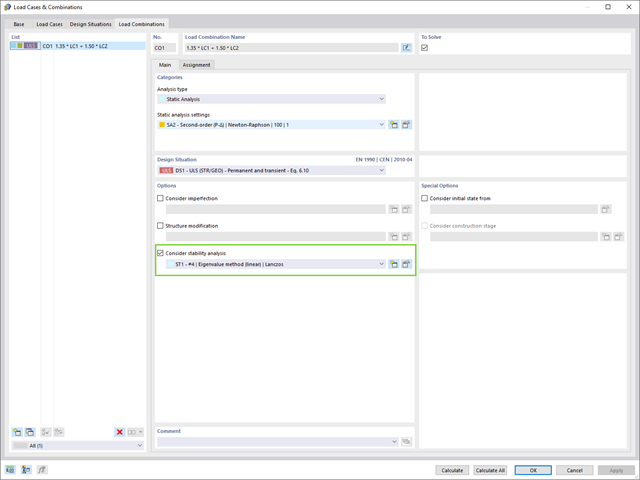
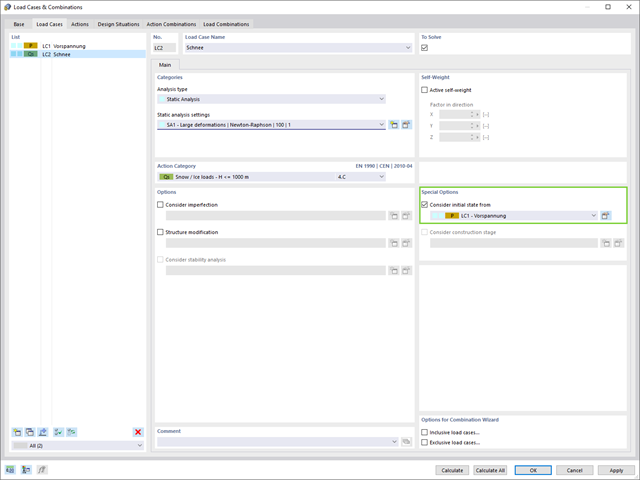
Jeżeli w programie istnieje przypadek obciążenia lub kombinacja obciążeń, obliczenia stateczności są aktywowane. Można zdefiniować inny przypadek obciążenia, na przykład w celu uwzględnienia naprężenia początkowego.
W tym celu należy określić, czy ma zostać przeprowadzona analiza liniowa czy nieliniowa. W zależności od przypadku zastosowania, można wybrać bezpośrednią metodę obliczeniową, taką jak metoda Lanczosa lub metoda iteracji ICG. Pręty niezintegrowane z powierzchniami są zazwyczaj wyświetlane jako elementy prętowe z dwoma węzłami ES. W przypadku zastosowania takich elementów program nie może określić wyboczenia lokalnego pojedynczych prętów. Z tego względu'istnieje możliwość automatycznego dzielenia prętów.
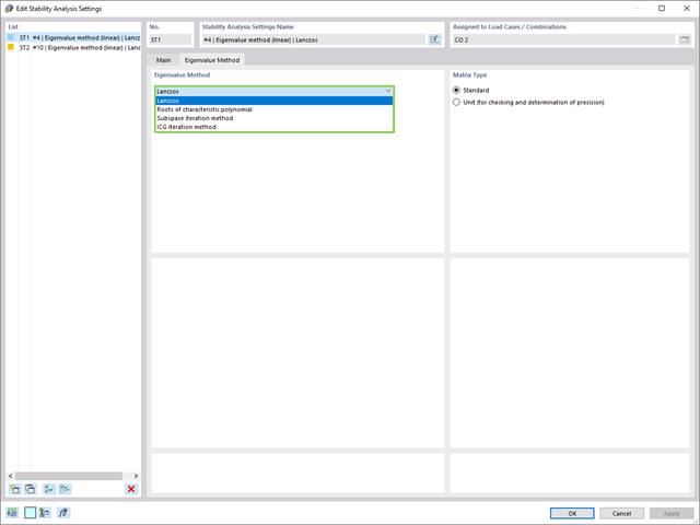
W przypadku analizy wartości własnych dostępnych jest kilka metod:
- Metody bezpośrednie
- Metody bezpośrednie (Lanczosa [RFEM], pierwiastki z wielomianu charakterystycznego [RFEM], metoda iteracji podprzestrzeni [RFEM/RSTAB], przesunięta iteracja odwrócona [RSTAB]) są odpowiednie dla małych i średnich modeli. Z szybkich metod rozwiązywania problemów należy korzystać tylko w przypadku, gdy komputer posiada dużą ilość pamięci RAM.
- Metoda iteracji ICG (niekompletny sprzężony gradient [RFEM])
- Z drugiej strony, ta metoda wymaga tylko niewielkiej ilości pamięci. Wartości własne są określane jedna po drugiej. Może być stosowany do obliczania dużych układów konstrukcyjnych o niewielkiej liczbie wartości własnych.
Rozszerzenie Stateczność konstrukcji umożliwia nieliniową analizę stateczności przy użyciu metody przyrostowej. Analiza ta dostarcza wyniki zbliżone do rzeczywistości również w przypadku konstrukcji nieliniowych. Współczynnik obciążenia krytycznego jest określany poprzez stopniowe zwiększanie obciążeń w podstawowym przypadku obciążenia, aż do osiągnięcia niestateczności. Przyrost obciążenia uwzględnia nieliniowości, takie jak ulegające uszkodzeniu pręty, podpory i fundamenty oraz nieliniowości materiałowe. Po zwiększeniu obciążenia można opcjonalnie przeprowadzić liniową analizę stateczności na ostatnim stabilnym stanie w celu określenia postaci stateczności.
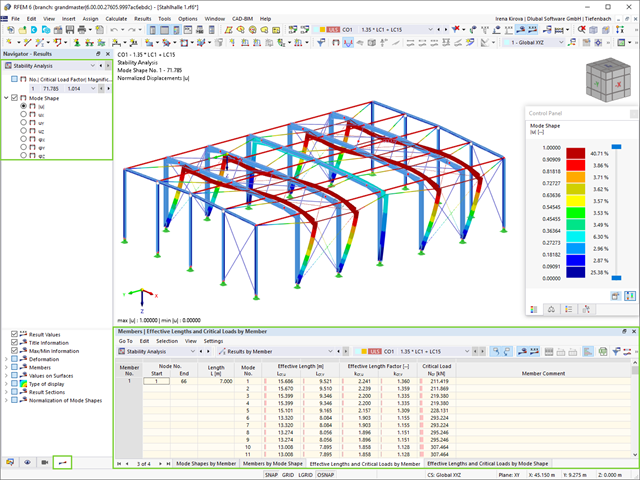
Jako pierwsze wyniki program przedstawia współczynniki obciążenia krytycznego. Następnie można przeprowadzić ocenę zagrożeń stateczności. W przypadku modeli prętowych w tabelach wyświetlane są wynikowe długości efektywne i obciążenia krytyczne prętów.
W następnym oknie wyników można sprawdzić znormalizowane wartości własne posortowane według węzła, pręta i powierzchni. Grafika wartości własnych umożliwia ocenę zachowania wyboczeniowego. Ułatwia to podjęcie środków zaradczych.
- 002073
- Ogólne informacje
- Analiza stateczności konstrukcji RFEM 6
- Analiza stateczności konstrukcji RSTAB 9
- Obliczanie modeli składających się z elementów prętowych, powłokowych i bryłowych
- Nieliniowa analiza stateczności
- Możliwość uwzględniania sił osiowych od wstępnego sprężenia
- Cztery dostępne solvery do rozwiązywania równań dla efektywnego obliczania różnych modeli konstrukcyjnych
- Opcjonalne uwzględnianie zmian w sztywności w programie RFEM/RSTAB
- Wyszukiwanie postaci wyboczeniowych o krytycznym mnożniku obciążenia większym niż zadany przez użytkownika (metoda "przesunięcia")
- Możliwość określania wektorów własnych dla modeli niestatecznych (w celu zidentyfikowania przyczyny niestateczności)
- Wizualizacja postaci niestateczności
- Podstawa określania imperfekcji
- Uwzględnianie i wyświetlanie mas kondygnacji
- Lista elementów konstrukcyjnych i ich informacje
- Automatyczne tworzenie przekrojów wynikowych na ścianach usztywniających
- Wyświetlanie wypadkowych przekrojów w kierunku globalnym do wyznaczania sił tnących
- Opcjonalna definicja sztywnej membrany według kondygnacji (modelowanie kondygnacji)
- Typ sztywności Płyta stropowa - tarcza sztywna
- Definiowanie zbiorów stropów,
- na przykład obliczanie płyt jako pozycji 2D w modelu 3D
- Ściany usztywniające: Automatyczne definiowanie prętów wynikowych o dowolnym przekroju
- Wymiarowanie przekrojów prostokątnych z wykorzystaniem rozszerzenia Projektowanie konstrukcji betonowych
- Definicja belek-ścian
- Wymiarowanie możliwe dzięki rozszerzeniu Projektowanie konstrukcji betonowych
- Tabelaryczne przedstawianie oddziaływań kondygnacji, znoszenia międzykondygnacyjnego oraz punktów środkowych masy i sztywności, jak również sił w ścianach usztywniających
- Oddzielne wyświetlanie wyników dla obliczeń stropu i usztywnień
- Opcjonalne pominięcie otworów o określonym rozmiarze
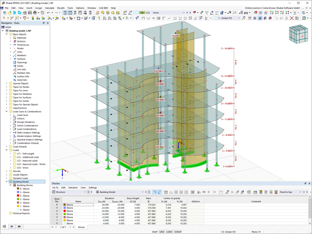
W przypadku modelu budynku dostępne są dwie opcje. Można go utworzyć na początku modelowania konstrukcji lub aktywować później. W modelu budynku można bezpośrednio definiować kondygnacje i modyfikować je.
Podczas manipulowania kondygnacjami można wybrać, czy zostaną zmodyfikowane, czy zachowane, korzystając z różnych opcji.
Program RFEM wykonuje część pracy za Ciebie. Na przykład, program automatycznie generuje przekroje wynikowe,'dzięki czemu nie trzeba wykonywać wielu obliczeń.
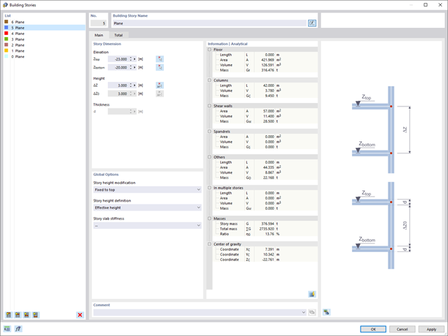
Wyniki można wyświetlić w zwykły sposób za pomocą nawigatora Wyniki. Ponadto w oknie dialogowym rozszerzenia wyświetlane są informacje o poszczególnych kondygnacjach. Dzięki temu zawsze masz dobry przegląd.
_ENG.png?mw=640&hash=1053c9bef400e9f5361c9c3278f76a272fcc4ddf)
Czy aktywowałeś rozszerzenie Analiza historii czasowej (TDA)? Dobrze, teraz można dodawać dane czasowe do przypadków obciążeń. Po zdefiniowaniu początku i końca obciążenia, uwzględniany jest wpływ pełzania na końcu obciążenia. Program umożliwia modelowanie efektów pełzania w konstrukcjach szkieletowych i kratowych wykonanych z betonu zbrojonego.
W tym przypadku obliczenia są przeprowadzane nieliniowo zgodnie z modelem reologicznym (model Kelvina i Maxwella).
Czy obliczenia zakończyły się pomyślnie? Wyznaczone siły wewnętrzne można teraz wyświetlić w tabelach i grafice, a także uwzględnić w obliczeniach.

- Definiowanie naprężeń na przykładzie sprężysto-plastycznego modelu materiałowego
- Wymiarowanie murowych konstrukcji tarczowych na ściskanie i ścinanie na modelu budynku lub na pojedynczym modelu
- Automatyczne określanie sztywności przegubu ściana-płyta
- Obszerna baza danych materiałów o prawie wszystkich kombinacjach kamienia i zapraw dostępnych na rynku austriackim (asortyment jest stale poszerzany, również dla innych krajów)
- Automatyczne określanie wartości materiałów zgodnie z Eurokodem 6 (ÖN EN 1996‑X)
- Możliwość przeprowadzenia analizy pushover
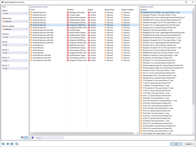
Konstrukcję wprowadza się i modeluje się bezpośrednio w programie RFEM. Model materiałowy muru można połączyć ze wszystkimi popularnymi rozszerzeniami dla programu RFEM. Umożliwia to projektowanie całych modeli budynków w połączeniu z murem.
Program automatycznie określa wszystkie parametry wymagane do obliczeń na podstawie wprowadzonych danych materiału. Następnie generowane są krzywe naprężenie-odkształcenie dla każdego elementu skończonego.
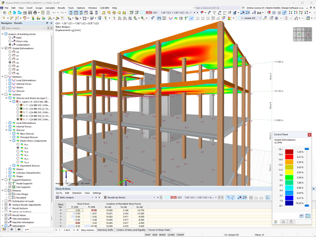
Czy projekt zakończył się sukcesem? Następnie po prostu usiądź i zrelaksuj się. Również tutaj można korzystać z licznych funkcji programu RFEM. Program podaje maksymalne naprężenia powierzchni murowanych, dzięki czemu można szczegółowo wyświetlić wyniki w każdym punkcie siatki ES.
Ponadto można wstawiać przekroje w celu przeprowadzenia szczegółowej analizy poszczególnych obszarów. Na podstawie przedstawionych obszarów uplastycznienia można oszacować zarysowania w murze.
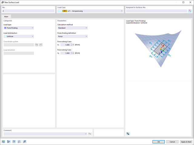
Po aktywowaniu rozszerzenia Form-Finding w Danych ogólnych, efekt znajdowania kształtu jest przypisywany do przypadków obciążeń z kategorią przypadków obciążenia "Sprężenie" w połączeniu z obciążeniami od znajdowania kształtu od pręta, powierzchni i bryły wczytaj katalog. Jest to przypadek obciążenia wstępnego naprężenia. Przekształca się on zatem w analizę znajdowania kształtu dla całego modelu ze zdefiniowanymi w nim wszystkimi elementami prętowymi, powierzchniowymi i bryłowymi. Do znajdowania kształtu odpowiednich elementów prętowych i membranowych dochodzi się w całym modelu za pomocą specjalnych obciążeń w zakresie znajdowania kształtu i regularnych definicji obciążeń. Te obciążenia znajdowania kształtu opisują oczekiwany stan odkształcenia lub siły po wyszukaniu kształtu w elementach. Obciążenia regularne opisują zewnętrzne obciążenie całego układu.
Czy wiesz dokładnie, w jaki sposób przebiega wyszukiwanie kształtu? Po pierwsze, proces znajdowania kształtu przypadków obciążeń z kategorią przypadku obciążenia "Wstępne naprężenie" przesuwa początkową geometrię siatki do optymalnie zrównoważonej pozycji za pomocą iteracyjnych pętli obliczeniowych. W tym celu program wykorzystuje metodę Zaktualizowanej Strategii Odniesienia (URS) opracowaną przez prof. Bletzingera i prof. Ramma. Technologię tę charakteryzują kształty równowagi, które po obliczeniach prawie dokładnie odpowiadają początkowo zadanym warunkom brzegowym (ugięcie, siła i naprężenie wstępne).
Oprócz opisu oczekiwanych sił lub zwisów na elementach, zintegrowane podejście URS umożliwia również uwzględnienie sił regularnych. W całym procesie pozwala to na przykład na opisanie ciężaru własnego lub ciśnienia pneumatycznego za pomocą odpowiednich obciążeń elementów.
Wszystkie te opcje dają rdzeniu obliczeniowemu możliwość obliczania postaci antyklastycznych i synklastycznych, które są w równowadze sił, dla geometrii płaskich lub obrotowo-symetrycznych. Aby możliwe było realistyczne zaimplementowanie obu typów, pojedynczo lub razem w jednym środowisku, w obliczeniach dostępne są dwa sposoby opisania wektorów sił do analizy form-finding:
- Metoda rozciągania - opis znajdowania kształtu wektorów sił w przestrzeni dla geometrii płaskich
- Metoda rzutowania - opis znajdowania kształtu wektorów sił na płaszczyznę rzutowania z ustaleniem położenia poziomego dla geometrii stożkowych
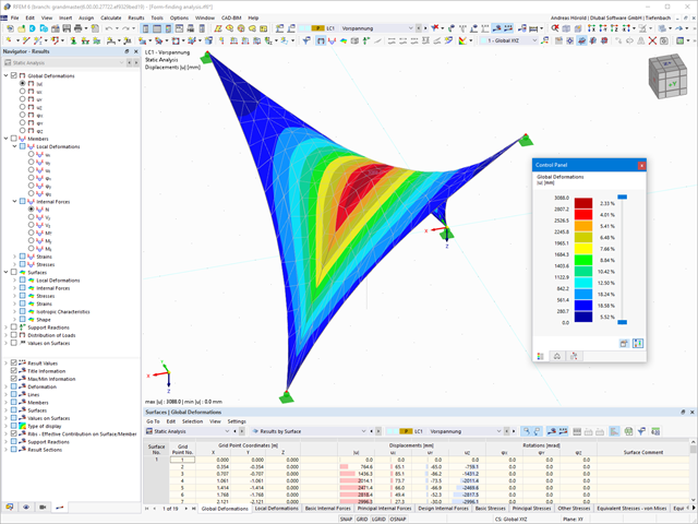
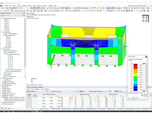
Proces znajdowania kształtu tworzy model konstrukcyjny z aktywnymi siłami w "przypadku obciążenia sprężonego" Ten przypadek obciążenia pokazuje przemieszczenie od początkowego położenia wejściowego do ustalonej geometrii w wynikach deformacji. W wynikach opartych na sile lub naprężeniach (siły wewnętrzne prętów i powierzchni, naprężenia w bryłach, ciśnienia gazu itp.) określany jest stan w celu zachowania znalezionej formy. Do analizy kształtu geometrycznego program oferuje dwuwymiarowy wykres konturowy z przedstawieniem wysokości bezwzględnej i wykresem nachylenia do wizualizacji sytuacji na zboczu.
Teraz przeprowadzane są dalsze obliczenia i analiza statyczno-wytrzymałościowa całego modelu. W tym celu program przenosi geometrię zorientowaną na kształt wraz z odkształceniami zależnymi od elementów do uniwersalnego stanu początkowego. Można go teraz używać w przypadkach obciążeń i kombinacjach obciążeń.
- 002162
- Ogólne informacje
- Analiza stateczności konstrukcji RFEM 6
- Analiza stateczności konstrukcji RSTAB 9
W porównaniu z modułami dodatkowymi RF-STABILITY (RFEM 5) i RSBUCK (RSTAB 8) do rozszerzenia Stateczność konstrukcji dla programu RFEM 6/RSTAB 9 dodano następujące nowe funkcje:
- Aktivierung als Eigenschaft eines Lastfalls oder einer Lastkombination
- Automatisierte Aktivierung der Stabilitätsberechnung über Kombinationsassistenten für mehrere Lastsituationen in einem Schritt
- Inkrementelle Laststeigerung mit benutzerdefinierten Abbruchkriterien
- Veränderung der Eigenformnormierung ohne Neuberechnung
- Ergebnistabellen mit Filteroption
W porównaniu z modułem dodatkowym RF-FORM-FINDING (RFEM 5), do modułu Form-Finding dla programu RFEM 6 dodano następujące nowe funkcje:
- Określenie wszystkich warunków brzegowych dotyczących obciążenia dla analizy znajdowania kształtu (form-finding) w pojedynczym przypadku obciążenia
- Przechowywanie wyników analizy znajdowania kształtu jako stanu początkowego z możliwością późniejszego wykorzystania przy dalszej analizie modelu
- Automatyczne przypisywanie stanu początkowego z analizy znajdowania kształtu do wszystkich sytuacji obciążeniowych w sytuacji obliczeniowej za pomocą kreatorów kombinacji
- Dodatkowe geometryczne warunki brzegowe dla prętów (długość elementu nieobciążonego, maksymalny zwis w pionie, zwis w pionie w najniższym punkcie punkcie)
- Dodatkowe warunki brzegowe z uwagi na obciążenie w analizie znajdowania kształtu dla prętów (maksymalna siła w pręcie, minimalna siła w pręcie, rozciągająca składowa pozioma, rozciąganie na i-końcu, rozciąganie na końcu j, minimalne rozciąganie na końcu i, minimalne rozciąganie na końcu j)
- Typ materiału „Tkanina” i „Folia” w bibliotece materiałów
- Równoległe analizy znajdowania kształtu w jednym modelu
- Symulacja kolejnych etapów znajdowania kształtów w połączeniu z rozszerzeniem Analiza etapów konstrukcji (CSA)

Dla każdego przypadku obciążenia można wyświetlić odkształcenia w czasie końcowym.
Wyniki te są również dokumentowane w protokole wydruku programów RFEM i RSTAB. Zawartość protokołu i jego zakres można wybrać specjalnie dla poszczególnych warunków projektowych.
Obawiasz się, że Twój projekt skończy się cyfrową wieżą Babel? Rozszerzenie Model budynku dla RFEM wspomaga pracę nad wielokondygnacyjnym projektem budowlanym. Tutaj możesz definiować i manipulować budynkiem za pomocą kondygnacji. Kondygnacje można później dostosować na wiele sposobów, a także wybrać sztywność płyty. Informacje na temat kondygnacji i całego modelu (środek ciężkości, środek sztywności) są wyświetlane w tabelach i na grafice.
Budowanie kamień na kamieniu ma długą tradycję w budownictwie. Rozszerzenie Projektowanie konstrukcji murowych dla RFEM umożliwia wymiarowanie konstrukcji murowych przy użyciu metody elementów skończonych. Rozszerzenie powstało w ramach projektu badawczego DDMaS - Digitalizacja wymiarowania konstrukcji murowych. Model materiałowy przedstawia nieliniowe zachowanie połączenia cegła-zaprawa w postaci modelowania w skali makro. Chcesz dowiedzieć się więcej?
Dzięki rozszerzeniu Analiza historii czasowej (TDA) można uwzględnić zmienne w czasie zachowanie materiału w przypadku prętów i powierzchni. Długotrwałe efekty, takie jak pełzanie, skurcz i starzenie, mogą wpływać na rozkład sił wewnętrznych, w zależności od konstrukcji. Darauf bereiten Sie sich mit diesem Add-On optimal vor.
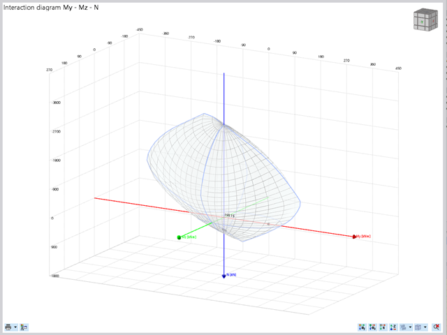
Projektowanie konstrukcji betonowych | Wykres interakcji My-Mz-N (3D) przekrojów z betonu zbrojonego
Na pytanie 'Ile można przewozić?' zazwyczaj odpowiada 'Tak'. Do graficznego przedstawiania stanu granicznego nośności przekrojów żelbetowych wymagany jest trójwymiarowy wykres interakcji momentu-momentu-siła osiowa. Oprogramowanie do analizy statyczno-wytrzymałościowej firmy Dlubal właśnie to oferuje.
Dzięki dodatkowemu wyświetleniu oddziaływania obciążenia można łatwo rozpoznać lub zwizualizować przekroczenie granicznej nośności przekroju żelbetowego. Ponieważ możesz kontrolować właściwości wykresu, możesz dostosować wygląd wykresu My-Mz-N do swoich potrzeb.
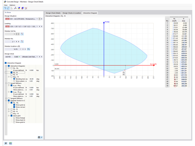
Czy wiesz, że wykresy interakcji moment-siła (wykresy MN) można wyświetlić również graficznie? Umożliwia to wyświetlenie nośności przekroju w przypadku interakcji momentu zginającego i siły osiowej. Oprócz wykresów interakcji związanych z osiami przekroju (wykres My-N i wykres Mz-N) można również wygenerować indywidualny wektor momentów w celu utworzenia wykresu interakcji Mres -N. Płaszczyznę przekroju wykresów MN można wyświetlić na wykresie interakcji 3D.Program wyświetla odpowiednie pary wartości stanu granicznego nośności w tabeli. Tabela jest dynamicznie powiązana z wykresem, dzięki czemu wybrany punkt graniczny jest również wyświetlany na wykresie.
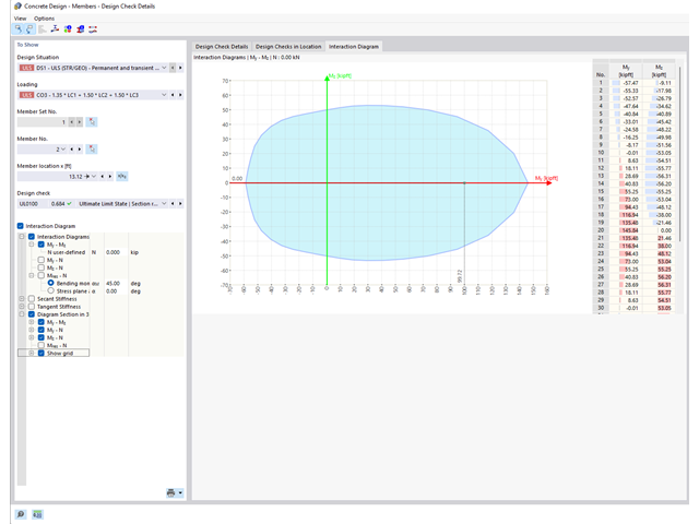
Czy chcesz określić nośność przekroju żelbetowego na zginanie dwukierunkowe? W tym celu należy najpierw aktywować wykres interakcji moment-moment (wykres My-Mz). Wykres My-Mz przedstawia poziomy przekrój przez trójwymiarowy wykres dla określonej siły osiowej N. Dzięki połączeniu z trójwymiarowym wykresem interakcji można tam również zwizualizować płaszczyznę przekroju.
.png?mw=640&hash=5a991f211d984ac624978f514e70c53da263e5d9)
W zależności od siły osiowej N, można wygenerować linię krzywizny momentu dla dowolnego wektora momentu. Program pokazuje również pary wartości wyświetlanego wykresu w tabeli. Ponadto można aktywować jako dodatkowy wykres sieczny i sztywność styczną przekroju żelbetowego, należące do wykresu krzywizny momentu.
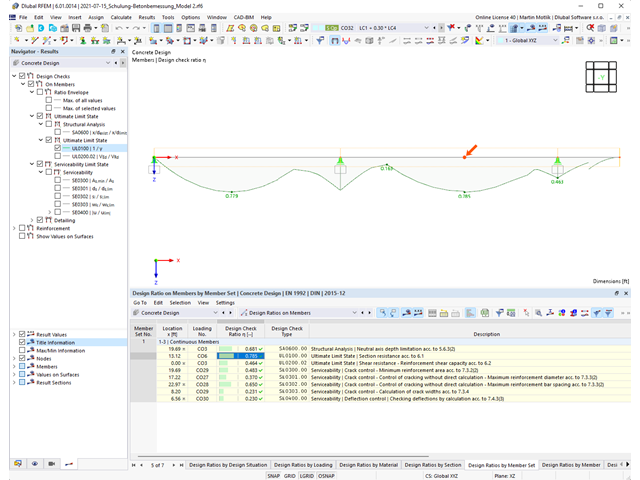
Program do analizy statyczno-wytrzymałościowej zapewnia przejrzysty przegląd wszystkich przeprowadzonych kontroli obliczeń dla określonej normy obliczeniowej. Dla każdego warunku projektowego należy określić kryterium obliczeniowe. Oprócz sprawdzania stanu granicznego nośności i użytkowalności program sprawdza zasady projektowania określone w normie. Dla każdej kontroli obliczeń są określone szczegóły obliczeń, w tym wartości początkowe, wyniki pośrednie i wyniki końcowe. Proces obliczeń wraz z zastosowanymi wzorami, standardowymi źródłami i wynikami szczegółowo przedstawiony jest w oknie informacyjnym w szczegółach obliczeń.
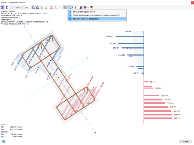
Istniejące naprężenia i odkształcenia przekroju betonowego i zbrojenia można wyświetlić w postaci obrazu naprężeń 3D lub grafiki 2D. W zależności od tego, które wyniki zostaną wybrane w drzewie wyników, naprężenia lub odkształcenia są wyświetlane w zdefiniowanym zbrojeniu podłużnym pod oddziaływaniami obciążeń lub granicznymi siłami wewnętrznymi.
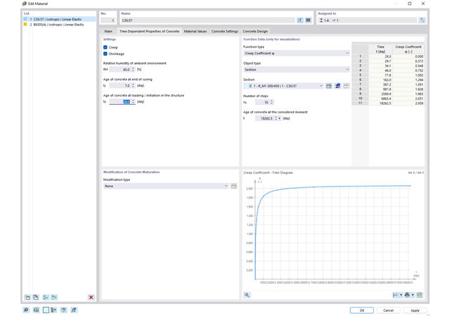
Właściwości betonu, zależne od czasu, takie jak pełzanie i skurcz, są bardzo ważne dla obliczeń. Można je zdefiniować bezpośrednio dla materiału w programie do analizy statyczno-wytrzymałościowej. W oknie dialogowym do wprowadzania danych wyświetlany jest przebieg czasowy funkcji pełzania lub skurczu. Można łatwo wybrać modyfikację zastosowanego wieku betonu, na przykład ze względu na obróbkę termiczną.
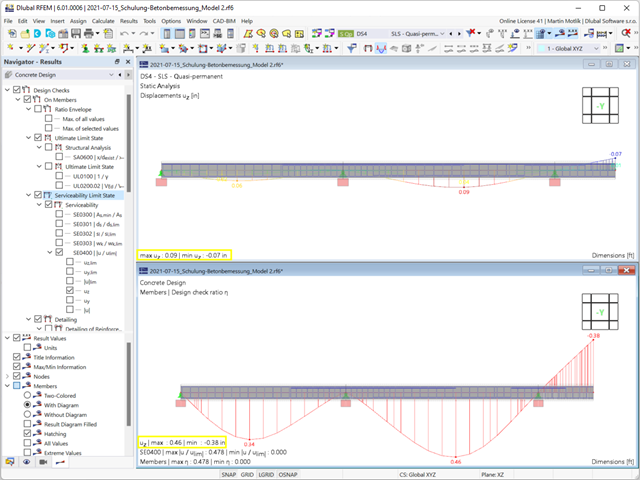
Odkształcenie prętów i powierzchni jest określane z uwzględnieniem zarysowanego (stan II) lub niezarysowanego (stan I) przekroju żelbetowego. Podczas określania sztywności można uwzględnić usztywnienie przy rozciąganiu między rysami, zwane 'usztywnieniem przy rozciąganiu', zgodnie z zastosowaną normą obliczeniową.
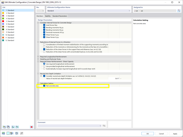
Podczas wymiarowania przekroju można bezpośrednio określić, czy powierzchnia betonowa zostanie zastosowana za prętami zbrojeniowymi, czy też zostanie odjęta od przekroju betonowego. Istnieje możliwość obliczenia przekroju betonu netto, zwłaszcza w przypadku przekroju silnie zbrojonego.
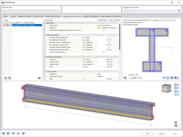
Zbrojenie na ścinanie i zbrojenie podłużne można zdefiniować indywidualnie dla każdego pręta. W tym przypadku dostępne są różne szablony do wprowadzania zbrojenia.