77 Wyniki
Wyświetl wyniki:
Sortuj według:
Parametry załączników krajowych (NA) do Eurokodu 3 z następujących krajów są zintegrowane:
-
 DIN EN 1993-1-1/NA:2016-04 (Niemcy)
 -
 ÖNORM EN 1993-1-1/NA:2015-12 (Austria)
 -
 SN EN 1993-1-1/NA:2016-07 (Szwajcaria)
 -
 BDS EN 1993-1-1/NA:2015-10 (Bułgaria)
 -
 BS EN 1993-1-1/NA:2016-07 (Wielka Brytania)
 -
 CEN EN 1993-1-1/2015-06 (Unia Europejska)
 -
 CYS EN 1993-1-1/NA:2015-07 (Cypr)
 -
 CSN EN 1993-1-1/NA:2016-06 (Republika Czeska)
 -
 DS EN 1993-1-1/NA:2015-07 (Dania)
 -
 ELOT EN 1993-1-1/NA:2017-01 (Grecja)
 -
 EVS EN 1993-1-1/NA:2015-08 (Estonia)
 -
 HRN EN 1993-1-1/NA:2016-03 (Chorwacja)
 -
 I S. EN 1993-1-1/NA:2016-03 (Irlandia)
 -
 ILNAS EN 1993-1-1/NA:2015-06 (Luksemburg)
 -
 IST EN 1993-1-1/NA:2015-11 (Islandia)
 -
 LST EN 1993-1-1/NA:2017-01 (Litwa)
 -
 LVS EN 1993-1-1/NA:2015-10 (Łotwa)
 -
 MS EN 1993-1-1/NA:2010-01 (Malezja)
 -
 MSZ EN 1993-1-1/NA:2015-11 (Węgry)
 -
 NBN EN 1993-1-1/NA:2015-07 (Belgia)
 -
 NEN EN 1993-1-1/NA:2016-12 (Holandia)
 -
 NF EN 1993-1-1/NA:2016-02 (Francja)
 -
 NP EN 1993-1-1/NA:2009-03 (Portugalia)
 -
 NS EN 1993-1-1/NA:2015-09 (Norwegia)
 -
 PN EN 1993-1-1/NA:2015-08 (Polska)
 -
 SFS EN 1993-1-1/NA:2015-08 (Finlandia)
 -
 SIST EN 1993-1-1/NA:2016-09 (Słowenia)
 -
 SR EN 1993-1-1/NA:2016-04 (Rumunia)
 -
 SS EN 1993-1-1/NA:2019-05 (Singapur)
 -
 SS EN 1993-1-1/NA:2015-06 (Szwecja)
 -
 STN EN 1993-1-1/NA:2015-10 (Słowacja)
 -
 TKP EN 1993-1-1/NA:2015-04 (Białoruś)
 -
 UNE EN 1993-1-1/NA:2016-02 (Hiszpania)
 -
 UNI EN 1993-1-1/NA:2015-08 (Włochy)
- Realistyczne odwzorowanie interakcji między budynkiem a gruntem
- Realistyczne odwzorowanie oddziaływania poszczególnych fundamentów na siebie nawzajem
- Biblioteka parametrów gruntowych z możliwością rozszerzania
- Możliwość uwzględniania wielu próbek gruntu z różnych lokalizacji, także poza obrysem budynku
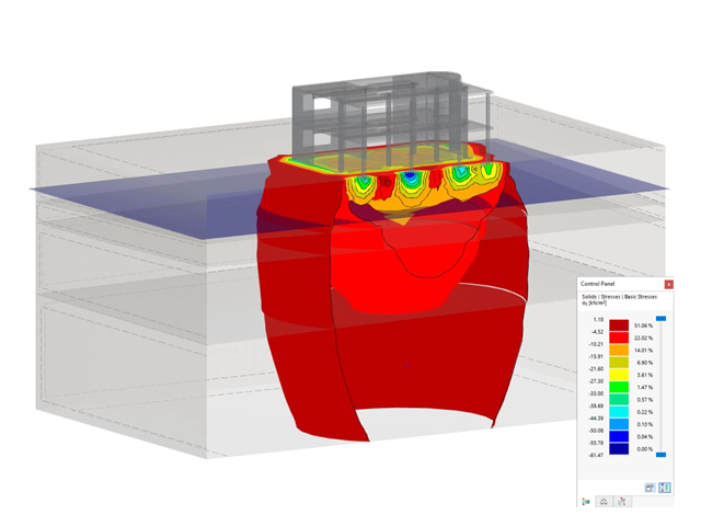
- Określanie osiadań oraz wykresów naprężeń w gruncie oraz ich prezentacja w formie graficznej i tabelarycznej

Wprowadzanie warstw gruntu dla potrzeb zadawania próbek gruntu odbywa się w przejrzystym oknie dialogowym. Odpowiadająca temu prezentacja graficzna zapewnia przejrzystość i ułatwia kontrolę wprowadzanych danych.
Rozszerzalna baza danych ułatwia wybór właściwości materiałowych dla gruntu. Dla realistycznego odwzorowania zachowania się materiału gruntowego można użyć modelu Mohra-Coulomba oraz model gruntu ze wzmocnieniem.
Można zdefiniować dowolną liczbę próbek i warstw gruntu. Grunt jest odwzorowany na podstawie wszystkich wprowadzonych próbek za pomocą brył 3D. Przypisanie do konstrukcji odbywa się za pomocą współrzędnych.
Zachowanie bryły gruntu jest obliczane za pomocą nieliniowej metody iteracyjnej. Obliczone naprężenia i osiadania są wyświetlane graficznie oraz w tabelach.
- Proste definiowanie etapów budowy konstrukcji w RFEM wraz z wizualizacją
- Dodawanie, usuwanie, modyfikowanie i reaktywacja elementów prętowych, powierzchniowych i bryłowych oraz ich właściwości (np. przeguby prętowe i liniowe, stopnie swobody dla podpór itp.)
- Ręczna oraz automatyczna kombinatoryka obciążeń na poszczególnych etapach budowy konstrukcji (np. w celu uwzględnienia obciążeń montażowych, tymczasowych urządzeń dźwigowych itp.)
- Uwzględnienie wpływów nieliniowych, takich jak uszkodzenie prętów rozciąganych lub nieliniowe zachowanie podpór
- Interakcja z innymi rozszerzeniami, takimi jak z. B. Nieliniowe zachowanie materiału, Stateczność konstrukcji, -rstab-9/additional-analyses/form-finding/form-finding itd.
- Wyświetlanie wyników w postaci numerycznej i graficznej dla poszczególnych etapów budowy
- Szczegółowy protokół wydruku wraz z dokumentacją wszystkich danych konstrukcyjnych i obciążeń dla każdego etapu budowy
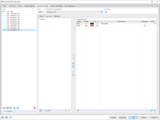
Czy udało Ci się utworzyć całą konstrukcję w programie RFEM? Dobrze, teraz można przypisać poszczególne elementy konstrukcyjne i przypadki obciążeń do odpowiednich etapów budowy. Na każdym etapie budowy można modyfikować na przykład definicje zwolnień prętów i podpór.
Pozwala to na modelowanie zmian konstrukcyjnych, na przykład podczas betonowania dźwigarów mostowych lub osiadania słupów. Przypadki obciążeń utworzone w programie RFEM należy następnie przydzielić do etapów budowy jako obciążenia stałe lub przejściowe.
Czy wiecie, że...? Kombinatoryka umożliwia nakładanie obciążeń stałych i przejściowych w kombinacjach obciążeń. W ten sposób można określić maksymalne siły wewnętrzne dla różnych pozycji dźwigu lub uwzględnić tymczasowe obciążenia montażowe dostępne tylko w jednym etapie budowy.
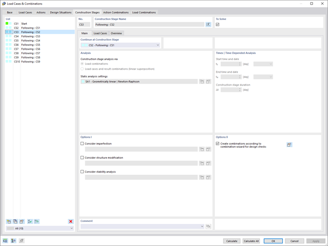
Jeżeli między idealnym układem a układem, który uległ deformacji z poprzedniego etapu budowy, pojawią się różnice w geometrii, są one porównywane w programie. Następujące po sobie kolejne etapy budowy obliczane są na bazie układu konstrukcyjnego z odkształceniami i obciążeniami wynikającymi z poprzednich etapu budowy. Obliczenia te są nieliniowe.
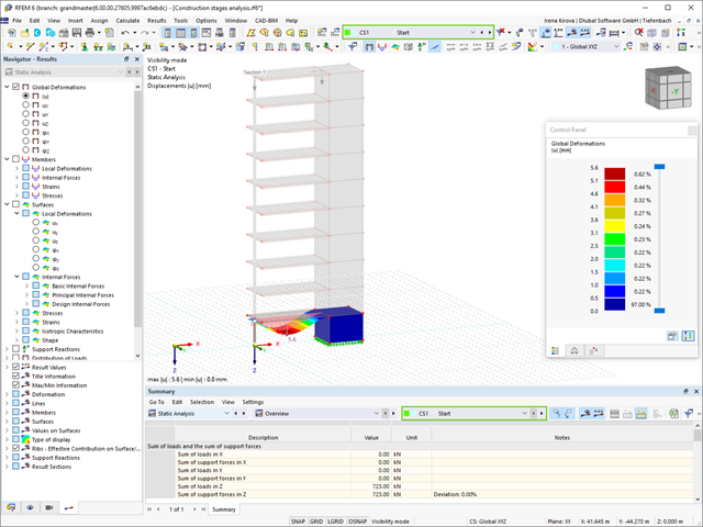
Czy obliczenia zakończyły się pomyślnie? Wyniki poszczególnych etapów budowy można teraz wyświetlać graficznie oraz w tabelach w programie RFEM. Ponadto program RFEM umożliwia uwzględnienie etapów budowy w kombinatoryce i uwzględnienie ich w dalszych obliczeniach.
_ENG.png?mw=640&hash=1053c9bef400e9f5361c9c3278f76a272fcc4ddf)
Czy aktywowałeś rozszerzenie Analiza historii czasowej (TDA)? Dobrze, teraz można dodawać dane czasowe do przypadków obciążeń. Po zdefiniowaniu początku i końca obciążenia, uwzględniany jest wpływ pełzania na końcu obciążenia. Program umożliwia modelowanie efektów pełzania w konstrukcjach szkieletowych i kratowych wykonanych z betonu zbrojonego.
W tym przypadku obliczenia są przeprowadzane nieliniowo zgodnie z modelem reologicznym (model Kelvina i Maxwella).
Czy obliczenia zakończyły się pomyślnie? Wyznaczone siły wewnętrzne można teraz wyświetlić w tabelach i grafice, a także uwzględnić w obliczeniach.
_(1).png?mw=640&hash=415f7bbaf70e41679bb0106e1cf91eaa8c493ec9)
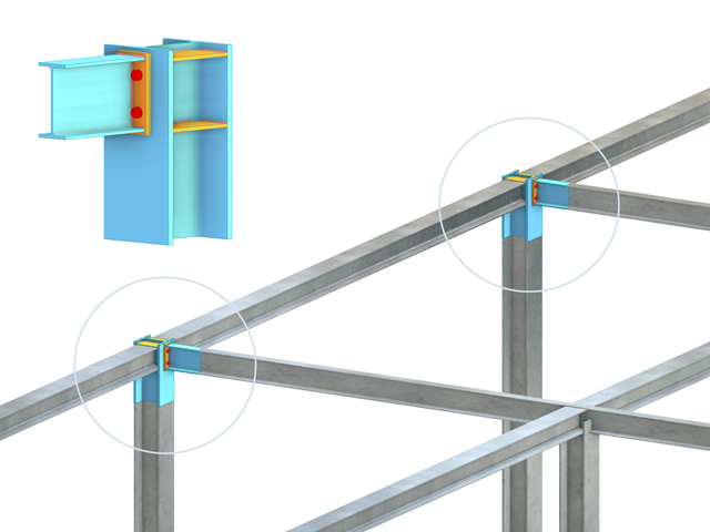
- Automatyczne generowanie modeli do analizy ES: rozszerzenie automatycznie tworzy w tle model elementów skończonych (ES) połączenia stalowego.
- Uwzględnienie wszystkich sił wewnętrznych: Obliczenia obejmują wszystkie siły wewnętrzne (N , Vy, Vz ,My, Mz, MT ) i nie są ograniczone do obciążeń płaskich.
- Automatyczne przenoszenie obciążeń: Wszystkie kombinacje obciążeń są automatycznie przenoszone do modelu analitycznego ES połączenia. Obciążenia są przenoszone bezpośrednio z programu RFEM, dzięki czemu ręczne wprowadzanie danych nie jest konieczne.
- Wydajne modelowanie: Rozszerzenie pozwala zaoszczędzić czas podczas modelowania złożonych sytuacji związanych z połączeniami. Utworzony model analityczny ES można również zapisać i wykorzystać do własnych szczegółowych analiz.
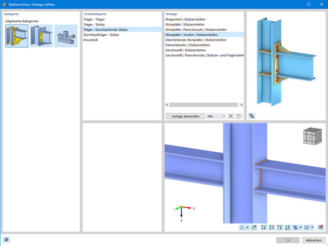
- Rozszerzalna biblioteka: Dostępna jest obszerna, rozszerzalna biblioteka zawierająca wstępnie zdefiniowane szablony połączeń stalowych.
- Szerokie zastosowanie: Rozszerzenie jest odpowiednie do tworzenia połączeń każdego typu i kształtu, jest kompatybilne z prawie wszystkimi przekrojami walcowanymi, spawanymi, złożonymi i cienkościennymi.
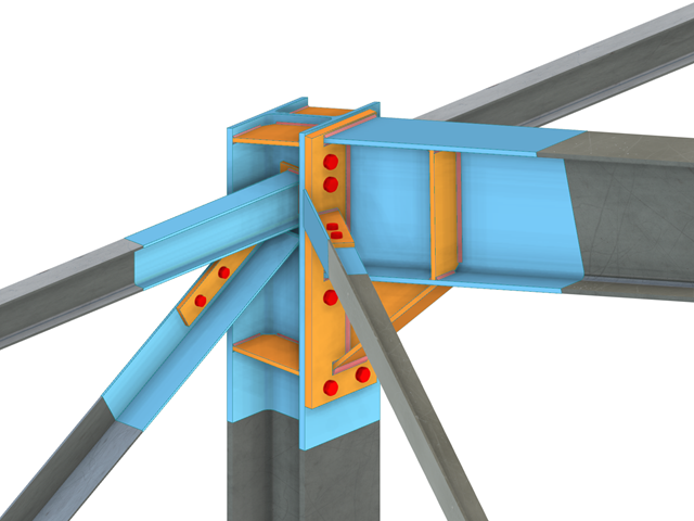
- Wybór węzłów w modelu RFEM, automatyczne rozpoznawanie i przydzielanie prętów połączonych z wybranym węzłem
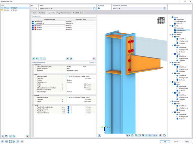
- Dostępnych jest wiele wstępnie zdefiniowanych elementów ułatwiających wprowadzanie typowych komponentów połączeń (np. blachy czołowe, żebra usztywniające)
- Uniwersalne komponenty bazowe (płyty, spoiny, płaszczyzny pomocnicze) do odwzorowania złożonych geometrii połączeń
- Użytkownik nie musi ręcznie edytować modelu MES połączenia, podstawowe ustawienia obliczeń można zmienić w oknie konfiguracji połączenia
- Automatyczne dostosowywanie geometrii połączenia, nawet w przypadku późniejszej edycji prętów, z uwagi na parametryczną definicję położenia komponentów względem siebie
- Równolegle do wprowadzania danych program przeprowadza kontrolę poprawności, aby szybko wykryć brakujące dane wejściowe lub kolizje elementów.
- Wizualizacja geometrii połączenia, która jest aktualizowana równolegle z wprowadzaniem danych
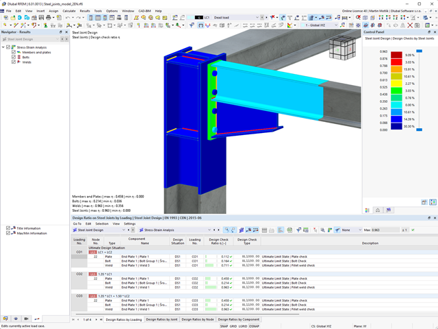
Program wspiera Cię: Moduł określa siły w śrubach na podstawie modelu analitycznego ES i analizuje je automatycznie. Rozszerzenie przeprowadza obliczenia nośności śrub dla przypadków uszkodzeń, takich jak rozciąganie, ścinanie, docisk otworu i przebicie, zgodnie z normą i wyświetla w przejrzysty sposób wszystkie wymagane współczynniki.
Chcesz przeprowadzić wymiarowanie spoin? Spoiny są modelowane jako sprężysto-plastyczne elementy powierzchniowe, a ich naprężenia są odczytywane z modelu analitycznego ES. Kryterium plastyczności ma reprezentować zniszczenie zgodnie z AISC J2-4, J2-5 (wytrzymałość spoin) i J2-2 (wytrzymałość metalu podstawowego). Obliczenia można przeprowadzić z zastosowaniem częściowych współczynników bezpieczeństwa określonych w załączniku krajowym do normy EN 1993-1-8.
Płyty w połączeniu są wymiarowane w sposób plastyczny poprzez porównanie istniejącego odkształcenia plastycznego z dopuszczalnym odkształceniem plastycznym. Domyślne ustawienie wynosi 5% zgodnie z EN 1993-1-5, Załącznik C, ale można to zmienić według specyfikacji użytkownika, a także 5% dla AISC 360.
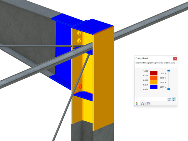
Wszystkie istotne wyniki można wyświetlić w modelu ES. W takim przypadku można filtrować wyniki osobno według odpowiednich komponentów.
Ponadto program RFEM zapewnia wszystkie kontrole obliczeń w formie tabelarycznej wraz z wyświetlaniem zastosowanych wzorów. W razie potrzeby tabele wyników można przenieść do protokołu wydruku programu RFEM.
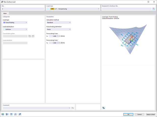
Po aktywowaniu rozszerzenia Form-Finding w Danych ogólnych, efekt znajdowania kształtu jest przypisywany do przypadków obciążeń z kategorią przypadków obciążenia "Sprężenie" w połączeniu z obciążeniami od znajdowania kształtu od pręta, powierzchni i bryły wczytaj katalog. Jest to przypadek obciążenia wstępnego naprężenia. Przekształca się on zatem w analizę znajdowania kształtu dla całego modelu ze zdefiniowanymi w nim wszystkimi elementami prętowymi, powierzchniowymi i bryłowymi. Do znajdowania kształtu odpowiednich elementów prętowych i membranowych dochodzi się w całym modelu za pomocą specjalnych obciążeń w zakresie znajdowania kształtu i regularnych definicji obciążeń. Te obciążenia znajdowania kształtu opisują oczekiwany stan odkształcenia lub siły po wyszukaniu kształtu w elementach. Obciążenia regularne opisują zewnętrzne obciążenie całego układu.
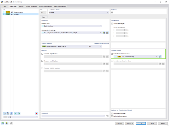
Czy wiesz dokładnie, w jaki sposób przebiega wyszukiwanie kształtu? Po pierwsze, proces znajdowania kształtu przypadków obciążeń z kategorią przypadku obciążenia "Wstępne naprężenie" przesuwa początkową geometrię siatki do optymalnie zrównoważonej pozycji za pomocą iteracyjnych pętli obliczeniowych. W tym celu program wykorzystuje metodę Zaktualizowanej Strategii Odniesienia (URS) opracowaną przez prof. Bletzingera i prof. Ramma. Technologię tę charakteryzują kształty równowagi, które po obliczeniach prawie dokładnie odpowiadają początkowo zadanym warunkom brzegowym (ugięcie, siła i naprężenie wstępne).
Oprócz opisu oczekiwanych sił lub zwisów na elementach, zintegrowane podejście URS umożliwia również uwzględnienie sił regularnych. W całym procesie pozwala to na przykład na opisanie ciężaru własnego lub ciśnienia pneumatycznego za pomocą odpowiednich obciążeń elementów.
Wszystkie te opcje dają rdzeniu obliczeniowemu możliwość obliczania postaci antyklastycznych i synklastycznych, które są w równowadze sił, dla geometrii płaskich lub obrotowo-symetrycznych. Aby możliwe było realistyczne zaimplementowanie obu typów, pojedynczo lub razem w jednym środowisku, w obliczeniach dostępne są dwa sposoby opisania wektorów sił do analizy form-finding:
- Metoda rozciągania - opis znajdowania kształtu wektorów sił w przestrzeni dla geometrii płaskich
- Metoda rzutowania - opis znajdowania kształtu wektorów sił na płaszczyznę rzutowania z ustaleniem położenia poziomego dla geometrii stożkowych
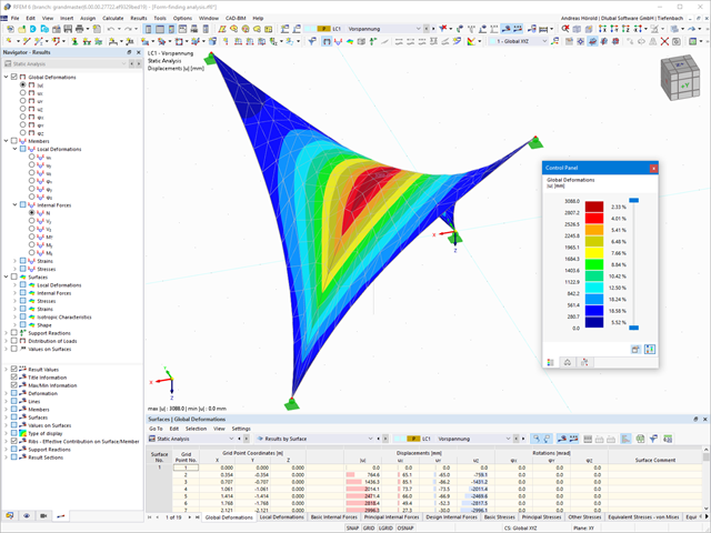
Proces znajdowania kształtu tworzy model konstrukcyjny z aktywnymi siłami w "przypadku obciążenia sprężonego" Ten przypadek obciążenia pokazuje przemieszczenie od początkowego położenia wejściowego do ustalonej geometrii w wynikach deformacji. W wynikach opartych na sile lub naprężeniach (siły wewnętrzne prętów i powierzchni, naprężenia w bryłach, ciśnienia gazu itp.) określany jest stan w celu zachowania znalezionej formy. Do analizy kształtu geometrycznego program oferuje dwuwymiarowy wykres konturowy z przedstawieniem wysokości bezwzględnej i wykresem nachylenia do wizualizacji sytuacji na zboczu.
Teraz przeprowadzane są dalsze obliczenia i analiza statyczno-wytrzymałościowa całego modelu. W tym celu program przenosi geometrię zorientowaną na kształt wraz z odkształceniami zależnymi od elementów do uniwersalnego stanu początkowego. Można go teraz używać w przypadkach obciążeń i kombinacjach obciążeń.
W porównaniu z modułem dodatkowym RF-/STAGES (RFEM 5) do rozszerzenia Analiza etapów budowy (CSA) dla programu RFEM 6 dodano następujące nowe funkcje:
- Uwzględnienie etapów budowy na poziomie programu RFEM
- Integracja analizy etapu budowy z kombinatoryką w programie RFEM
- Wprowadzono podparcie dla dodatkowych elementów konstrukcyjnych, takich jak przeguby liniowe
- Analiza alternatywnych procesów konstrukcyjnych w modelu
- Ponowna aktywacja elementów konstrukcyjnych
W porównaniu z modułem dodatkowym RF-FORM-FINDING (RFEM 5), do modułu Form-Finding dla programu RFEM 6 dodano następujące nowe funkcje:
- Określenie wszystkich warunków brzegowych dotyczących obciążenia dla analizy znajdowania kształtu (form-finding) w pojedynczym przypadku obciążenia
- Przechowywanie wyników analizy znajdowania kształtu jako stanu początkowego z możliwością późniejszego wykorzystania przy dalszej analizie modelu
- Automatyczne przypisywanie stanu początkowego z analizy znajdowania kształtu do wszystkich sytuacji obciążeniowych w sytuacji obliczeniowej za pomocą kreatorów kombinacji
- Dodatkowe geometryczne warunki brzegowe dla prętów (długość elementu nieobciążonego, maksymalny zwis w pionie, zwis w pionie w najniższym punkcie punkcie)
- Dodatkowe warunki brzegowe z uwagi na obciążenie w analizie znajdowania kształtu dla prętów (maksymalna siła w pręcie, minimalna siła w pręcie, rozciągająca składowa pozioma, rozciąganie na i-końcu, rozciąganie na końcu j, minimalne rozciąganie na końcu i, minimalne rozciąganie na końcu j)
- Typ materiału „Tkanina” i „Folia” w bibliotece materiałów
- Równoległe analizy znajdowania kształtu w jednym modelu
- Symulacja kolejnych etapów znajdowania kształtów w połączeniu z rozszerzeniem Analiza etapów konstrukcji (CSA)
W porównaniu z modułem dodatkowym RF-SOILIN (RFEM 5) do rozszerzenia Analiza geotechniczna dla programu RFEM 6 dodano następujące nowe funkcje:
- Tworzenie warstwowego gruntu jako modelu 3D z całości zdefiniowanych próbek gruntu
- Symulacja gruntu zgodnie z teorią Mohra-Coulomba
- Graficzne i tabelaryczne przedstawienie naprężeń i odkształceń na dowolnej głębokości gruntu
- Optymalne uwzględnienie interakcji gruntu i konstrukcji na podstawie modelu ogólnego

Dla każdego przypadku obciążenia można wyświetlić odkształcenia w czasie końcowym.
Wyniki te są również dokumentowane w protokole wydruku programów RFEM i RSTAB. Zawartość protokołu i jego zakres można wybrać specjalnie dla poszczególnych warunków projektowych.
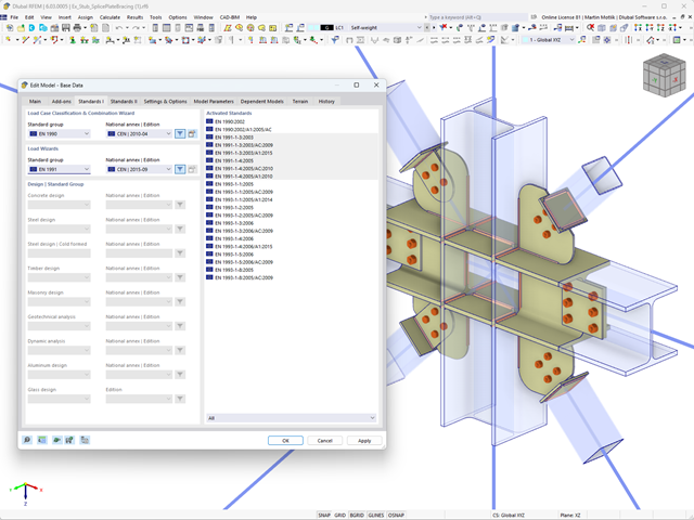
Pracujesz z połączeniami stalowymi? Rozszerzenie Połączenia stalowe dla programu RFEM ułatwia analizę połączeń stalowych za pomocą modelu ES. Modelowanie przebiega całkowicie automatycznie w tle. Proces można jednak kontrolować poprzez proste i wygodne wprowadzanie elementów. Następnie należy wykorzystać naprężenia określone w modelu ES do wymiarowania elementów zgodnie z EN 1993-1-8 (wraz z załącznikami krajowymi).
Dzięki rozszerzeniu Analiza historii czasowej (TDA) można uwzględnić zmienne w czasie zachowanie materiału w przypadku prętów i powierzchni. Długotrwałe efekty, takie jak pełzanie, skurcz i starzenie, mogą wpływać na rozkład sił wewnętrznych, w zależności od konstrukcji. Darauf bereiten Sie sich mit diesem Add-On optimal vor.
W przypadku elementów połączenia można sprawdzić, czy utrata stateczności jest istotna. Wymaga to rozszerzenia Stateczność konstrukcji.
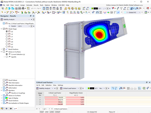
Współczynnik obciążenia krytycznego obliczany jest dla wszystkich analizowanych kombinacji obciążeń oraz wybranej liczby postaci własnych dla modelu połączenia. Porównaj najmniejszy współczynnik obciążenia krytycznego z wartością graniczną 15 z normy EN 1993-1-1, rozdz. 5. Ponadto użytkownik może samodzielnie dostosować wartość graniczną. Wynikiem analizy stateczności jest wyświetlenie w programie graficznej postaci odpowiednich postaci drgań.
Na potrzeby analizy stateczności dostosowany model powierzchniowy jest wykorzystywany w programie RFEM do rozpoznania lokalnych kształtów wyboczeniowych. Można również zapisać model analizy stateczności wraz z wynikami i wykorzystać jako osobny plik modelu.
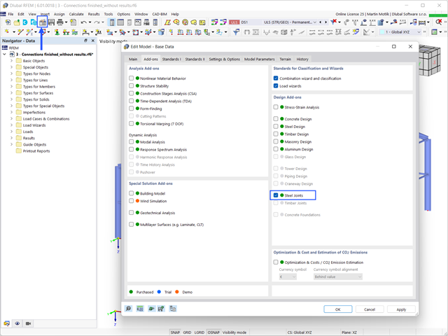
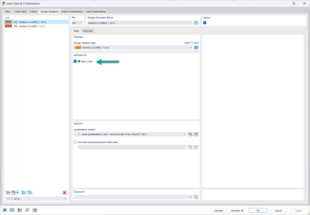
Aby zwymiarować połączenie stalowe, należy aktywować rozszerzenie Połączenia stalowe. Rozszerzenia w programie RFEM 6 są aktywowane w zakładce Rozszerzenia w oknie Edytować model - dane podstawowe. Jeżeli rozszerzenie jest aktywne, jest wyświetlane w nawigatorze.
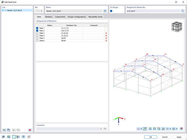
- W przypadku nowego modelu połączenia należy wybrać węzeł w modelu RFEM
- Po wybraniu węzła pręty połączone z węzłem są automatycznie rozpoznawane i przydzielane
- W oknie służącym do przydzielania prętów należy wybrać pręty, które zostaną przydzielone do połączenia
- Zaznaczone przez nas pręty są wyświetlane w oknie podglądu po prawej stronie
- Połączenia mogą być modelowane dla wielu węzłów w konstrukcji.
- Jako ustawienia prętów należy wybrać te, które mają być podparte
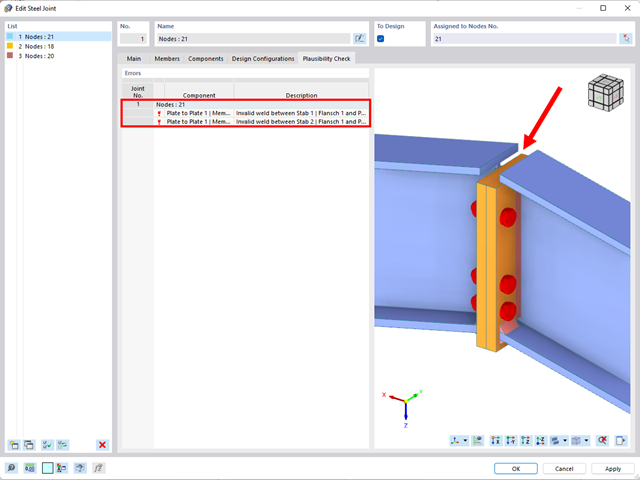
- Równolegle do wprowadzania danych program przeprowadza kontrolę poprawności, aby szybko wykryć brakujące dane wejściowe lub kolizje.
- W przypadku błędu pojawia się komunikat opisujący problem.
- Model połączeń stalowych i wyniki można zapisać jako osobny plik modelu
- Uzyskane naprężenia i wyniki analizy stateczności (wyboczenia połączenia) można wyświetlić w osobnym modelu
- W zapisanym modelu można uruchomić animację deformacji połączenia
- Elementy połączenia są podczas zapisywania przekształcane w powierzchnie i pręty
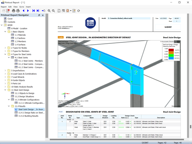
- Wyniki wymiarowania połączeń można wprowadzić do protokołu wydruku
- Podczas tworzenia nowego protokołu wydruku należy wybrać elementy dodane z rozszerzenia Połączenia stalowe
- Za pomocą narzędzia 'Drukowanie grafik do protokołu' można wstawić do protokołu grafikę z wynikami połączenia, w tym z panelem sterowania.
- Protokół wydruku zawiera specyfikacje elementów połączenia, parametry obliczeniowe, wyniki i grafiki
- Proponowane połączenie można zastosować do wszystkich wybranych węzłów w konstrukcji
- Położenie połączenia można zdefiniować w zakładce 'Główne' okna dialogowego rozszerzenia
- Obliczenia są przeprowadzane dla wszystkich połączeń w konstrukcji, a po zakończeniu obliczeń wyniki mogą być wyświetlane we wszystkich połączeniach
- W tabeli wyświetlane są wyniki dla poszczególnych połączeń, każde połączenie jest obliczane i może być zapisane osobno
- Elementy łączące są obliczane zgodnie z AISC 360-16 i Eurokodem EN 1993-1-8.
- Po aktywacji rozszerzenia sytuacje obliczeniowe dla połączeń stalowych należy aktywować w oknie dialogowym „Przypadki obciążeń i kombinacje”.
- Do obliczenia stateczności (wyboczenia) połączenia wymagane jest rozszerzenie 'Stateczność konstrukcji'.
- Obliczenia można uruchomić za pomocą tabeli lub ikony w górnym pasku.
Wymiarowanie połączenia ramy o prętach zbieżnych i usztywnionych. Dla połączenia przeprowadzono analizę naprężeń i stateczności przy wyboczeniu. Aby wyświetlić wyniki dla wyboczenia, połączenie zostało przekształcone w osobny model.