62 Wyniki
Wyświetl wyniki:
Sortuj według:
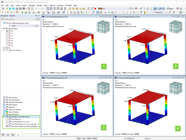
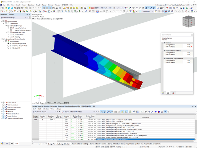
Jak już wiesz, po pomyślnym zakończeniu obliczeń wyniki przypadku obciążenia w Analizie modalnej są wyświetlane w programie. Die erste Eigenform ist für Sie also sofort grafisch oder animiert zu sehen. Dabei können Sie die Darstellung der Eigenformnormierung komfortabel anpassen. Erledigen Sie das am besten direkt im Ergebnisnavigator, wo Sie zur Visualisierung der Eigenformen eine von vier Optionen auswählen:
- Wert des Eigenformvektors uj auf 1 skalieren (berücksichtigt nur die Translationskomponenten)
- Auswahl der maximalen Translationskomponente des Eigenvektors und Einstellung auf 1
- Betrachtung der gesamten Eigenform (inklusive der Rotationskomponenten), Auswahl des Maximums und Einstellung auf 1
- Setzen der modalen Massen mi für jeden Eigenwert auf 1 kg
Ausführlichere Erläuterungen der Normierung der Eigenformen finden Sie hier: Instrukcja online .
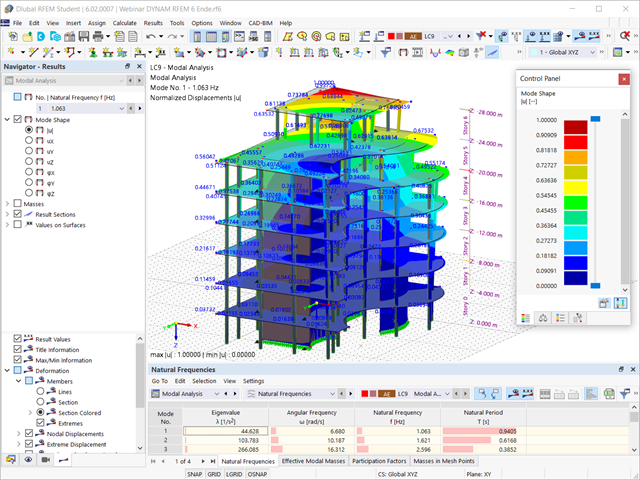
Czy obliczenia się zakończyły? Wyniki analizy modalnej są wówczas dostępne zarówno w formie graficznej, jak i tabelarycznej. Wyświetl tabele wyników dla przypadku obciążenia lub przypadków obciążeń analizy modalnej. Dzięki temu na pierwszy rzut oka można zobaczyć wartości własne, częstotliwości kątowe, częstotliwości i okresy drgań własnych konstrukcji. W przejrzysty sposób wyświetlane są również efektywne masy modalne, modalne współczynniki masy i współczynniki udziału.
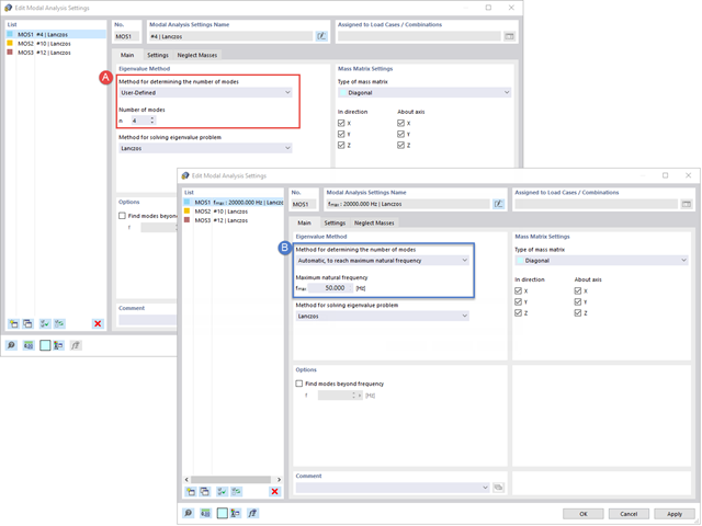
Twoim celem jest określenie liczby postaci drgań własnych? Program oferuje dwie metody. Z jednej strony, można ręcznie zdefiniować liczbę najmniejszych kształtów drgań, które mają zostać obliczone. W tym przypadku liczba dostępnych kształtów postaci zależy od stopni swobody (tzn. liczby punktów mas swobodnych pomnożonych przez liczbę kierunków, w których działają masy). Jest to jednak ograniczone do 9999. Z drugiej strony, maksymalną częstotliwość drgań własnych można ustawić w taki sposób, w jaki program określił kształty automatycznie, aż do osiągnięcia zadanej częstotliwości drgań własnych.
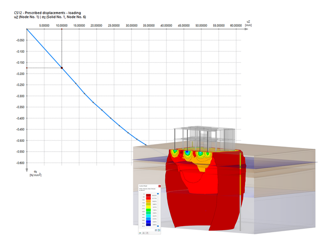
Czy jesteś gotowy na ocenę? Skorzystaj z wykresów obliczeniowych, które pokazują rozkład określonego wyniku podczas obliczeń.
Przypisanie osi pionowej i poziomej wykresu obliczeniowego można dowolnie definiować. Umożliwia to np. wyświetlenie przebiegu osiadania określonego węzła w zależności od obciążenia.
- 002462
- Ogólne informacje
- Projektowanie konstrukcji aluminiowych RFEM 6
- Projektowanie konstrukcji aluminiowych RSTAB 9
Czy do określenia współczynnika obciążenia krytycznego w ramach analizy stateczności użyto dodatkowego solwera wewnętrznych wartości własnych? W takim przypadku można następnie wyświetlić kształt wzorca projektowanego obiektu.
- 002457
- Ogólne informacje
- Projektowanie konstrukcji aluminiowych RFEM 6
- Projektowanie konstrukcji aluminiowych RSTAB 9
Rozszerzenie Projektowanie konstrukcji aluminiowych oferuje dodatkowe opcje. W tym miejscu można również obliczać przekroje ogólne, które nie są wstępnie zdefiniowane w bibliotece przekrojów. Na przykład, utwórz przekrój w programie RSECTION, a następnie zaimportuj go do RFEM/RSTAB. W zależności od zastosowanej normy projektowej dostępne są różne formaty obliczeń. Obejmuje to na przykład równoważną analizę naprężeń.
Ist zudem eine Lizenz für RSECTION und „Effektive Querschnitte“ vorhanden, so können Sie die Nachweise auch unter Berücksichtigung der effektiven Querschnittswerte nach EN 1999-1-1 führen.
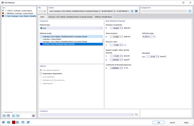
Czy chcesz modelować i analizować zachowanie bryły gruntowej? Aby to zapewnić, w programie RFEM zaimplementowano odpowiednie modele materiałowe.
Można użyć zmodyfikowanego modelu Mohra-Coulomba z liniowo-sprężystym modelem idealnie plastycznym lub nieliniowo sprężystym modelem z edometryczną relacją naprężenie-odkształcenie. Kryterium graniczne, które opisuje przejście od obszaru sprężystości do obszaru płynięcia plastycznego, jest zdefiniowane według Mohra-Coulomba.
W rozszerzeniu Projektowanie konstrukcji betonowych można przeprowadzać obliczenia sejsmiczne dla prętów żelbetowych zgodnie z EC 8. Są to między innymi następujące funkcje:
- Konfiguracje obliczeń sejsmicznych
- Rozróżnianie klas ciągliwości DCL, DCM, DCH
- Możliwość przeniesienia współczynnika odpowiedzi z analizy dynamicznej
- Sprawdzenie wartości granicznej współczynnika odpowiedzi
- Weryfikacja nośności dla "Wytrzymały słup - słaba belka"
- Uszczegółowienie i reguły szczególne dla współczynnika ciągliwości krzywizny
- Uszczegółowienie i reguły szczególne dla ciągliwości lokalnej
.png?mw=640&hash=403c565ab80c4dd45c2d1356634fb74a90428b70)
W bibliotece konstrukcji warstwowych dostępni są następujący producenci drewna klejonego krzyżowo:
- Binderholz (USA)
- KLH (USA, CAN)
- Kalesnikoff (USA, CAN)
- Nordic Structures (USA, CAN)
- Mercer Mass Timber
- SmartLam
- Sterling Structural
- Konstrukcje nośne wymienione w Lignatec wydanie 32 "Drewno klejone krzyżowo z produkcji szwajcarskiej"
Wczytanie konstrukcji z biblioteki konstrukcji warstw powoduje automatyczne przejęcie wszystkich istotnych parametrów. Biblioteka jest stale aktualizowana.

W porównaniu z modułem dodatkowym RF-SOILIN (RFEM 5) do rozszerzenia Analiza geotechniczna dla programu RFEM 6 dodano następujące nowe funkcje:
- Tworzenie warstwowego gruntu jako modelu 3D z całości zdefiniowanych próbek gruntu
- Symulacja gruntu zgodnie z teorią Mohra-Coulomba
- Graficzne i tabelaryczne przedstawienie naprężeń i odkształceń na dowolnej głębokości gruntu
- Optymalne uwzględnienie interakcji gruntu i konstrukcji na podstawie modelu ogólnego
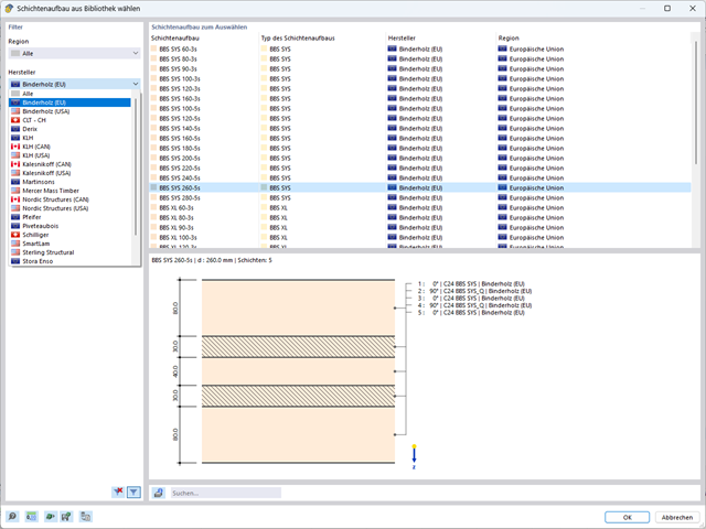
W programie RFEM zaimplementowano bibliotekę płyt z drewna klejonego krzyżowo, z której można importować konstrukcje warstwowe różnych producentów (np. Binderholz, KLH, Piveteaubois, Södra, Züblin Timber, Schilliger, Stora Enso). Oprócz grubości i materiałów warstw podane są również informacje o redukcji sztywności i łączeniu wąskich boków.
Przejdź do filmu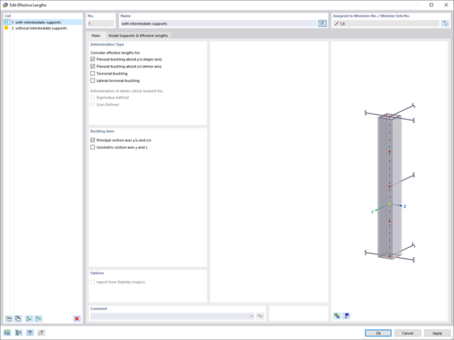
- 002142
- Wyniki
- Projektowanie konstrukcji aluminiowych RFEM 6
- Projektowanie konstrukcji aluminiowych RSTAB 9
- Analiza stateczności dla wyboczenia giętnego, wyboczenia skrętnego i wyboczenia giętno-skrętnego przy ściskaniu
- Analiza zwichrzenia elementów poddanych obciążeniu momentem
- Import długości efektywnych z obliczeń przy użyciu rozszerzenia Stateczność konstrukcji
- Graficzne wprowadzanie i kontrola zdefiniowanych podpór węzłowych oraz długości efektywnych w celu analizy stateczności
- W zależności od normy istnieje wybór między wprowadzaniem wartości Mcr przez użytkownika, metodą analityczną z normy lub wykorzystaniem wewnętrznego solwera wartości własnych
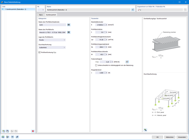
- Uwzględnienie panelu usztywniającego i ograniczenia obrotu podczas korzystania z solwera wartości własnych
- Graficzne przedstawienie postaci własnej w przypadku zastosowania solwera wartości własnych
- Analiza stateczności elementów konstrukcyjnych ze ściskaniem i naprężeniem zginającym, w zależności od normy obliczeniowej
- Przejrzyste obliczanie wszystkich niezbędnych współczynników, takich jak współczynniki interakcji
- Alternatywne uwzględnienie wszystkich wpływów dla analizy stateczności podczas określania sił wewnętrznych w programie RFEM/RSTAB (analiza drugiego rzędu, imperfekcje, redukcja sztywności, ewentualnie w połączeniu z rozszerzeniem Skręcanie skrępowane (7 stopni swobody))
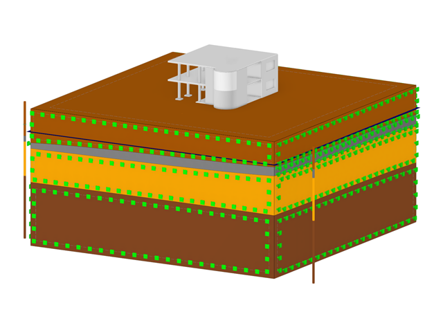
Bryły gruntu, które mają zostać przeanalizowane, są sumowane w masywach gruntu.
Próbki gruntu należy wykorzystać jako podstawę do zdefiniowania masywu gruntowego. W ten sposób program umożliwia generowanie masywu w sposób przyjazny dla użytkownika, w tym automatyczne określanie granic faz na podstawie danych z próbki, a także poziomu wód gruntowych i podpór powierzchni granicznej.
Masywy gruntowe umożliwiają określenie docelowego rozmiaru siatki ES niezależnie od ustawień globalnych dla reszty konstrukcji. Dzięki temu w całym modelu można uwzględnić różne wymagania dotyczące budynku i gruntu.
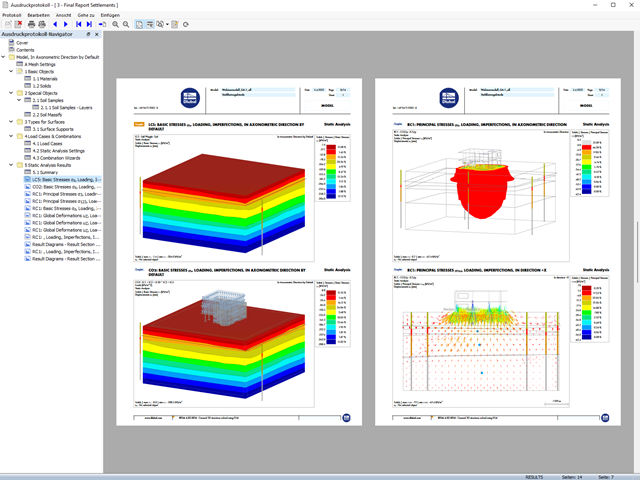
Twoje dane są zawsze dokumentowane w wielojęzycznym raporcie. W każdej chwili możesz dostosować treść i zapisać ją jako szablon. W raporcie można również za pomocą kilku kliknięć umieścić grafiki, teksty, wzory MathML i dokumenty PDF.
- 002173
- Ogólne informacje
- Projektowanie konstrukcji aluminiowych RFEM 6
- Projektowanie konstrukcji aluminiowych RSTAB 9
W porównaniu z modułem dodatkowym RF-/ALUMINIUM (RFEM 5/RSTAB 8) do rozszerzenia Projektowanie konstrukcji aluminiowych dla programu RFEM 6/RSTAB 9 dodano następujące nowe funkcje:
- Oprócz Eurokodu 9, dostępna jest amerykańska norma ADM 2020.
- Uwzględnienie stabilizującego efektu płatwi i blachy trapezowej za pomocą podparcia obrotowych stopni swobody oraz paneli usztywniających
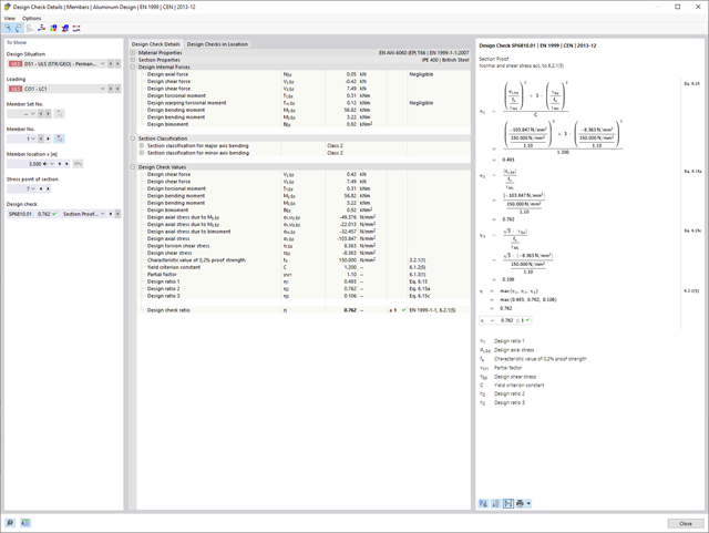
- Graficzne przedstawienie wyników na przekroju brutto
- Wyświetlanie odpowiednich wzorów użytych do sprawdzania warunków nośności (w tym odniesienie do zastosowanego równania z normy)
- 002459
- Ogólne informacje
- Projektowanie konstrukcji aluminiowych RFEM 6
- Projektowanie konstrukcji aluminiowych RSTAB 9
Rozszerzenie Skręcanie skrępowane (7 stopni swobody) umożliwia przeprowadzanie obliczeń konstrukcji prętowych w programach RFEM i RSTAB, z uwzględnieniem deplanacji przekrojów. Wszystkie siły wewnętrzne (N, Vu, Vv, Mt, pri, Mt, sec, Mu, Mv, Mω) określone w ten sposób mogą zostać uwzględnione w analizie naprężeń zastępczych dla obliczeń konstrukcji aluminiowych. Uwaga: Ta funkcja nie jest jeszcze dostępna dla norm projektowych ADM 2020.
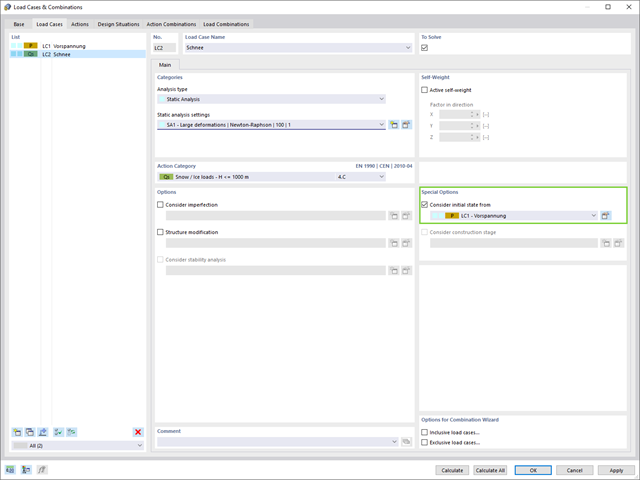
Czy wiesz dokładnie, w jaki sposób przebiega wyszukiwanie kształtu? Po pierwsze, proces znajdowania kształtu przypadków obciążeń z kategorią przypadku obciążenia "Wstępne naprężenie" przesuwa początkową geometrię siatki do optymalnie zrównoważonej pozycji za pomocą iteracyjnych pętli obliczeniowych. W tym celu program wykorzystuje metodę Zaktualizowanej Strategii Odniesienia (URS) opracowaną przez prof. Bletzingera i prof. Ramma. Technologię tę charakteryzują kształty równowagi, które po obliczeniach prawie dokładnie odpowiadają początkowo zadanym warunkom brzegowym (ugięcie, siła i naprężenie wstępne).
Oprócz opisu oczekiwanych sił lub zwisów na elementach, zintegrowane podejście URS umożliwia również uwzględnienie sił regularnych. W całym procesie pozwala to na przykład na opisanie ciężaru własnego lub ciśnienia pneumatycznego za pomocą odpowiednich obciążeń elementów.
Wszystkie te opcje dają rdzeniu obliczeniowemu możliwość obliczania postaci antyklastycznych i synklastycznych, które są w równowadze sił, dla geometrii płaskich lub obrotowo-symetrycznych. Aby możliwe było realistyczne zaimplementowanie obu typów, pojedynczo lub razem w jednym środowisku, w obliczeniach dostępne są dwa sposoby opisania wektorów sił do analizy form-finding:
- Metoda rozciągania - opis znajdowania kształtu wektorów sił w przestrzeni dla geometrii płaskich
- Metoda rzutowania - opis znajdowania kształtu wektorów sił na płaszczyznę rzutowania z ustaleniem położenia poziomego dla geometrii stożkowych
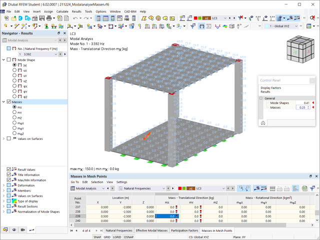
Czy odkryłeś już tabelaryczne i graficzne przedstawianie mas w punktach siatki? Po prawej, jest to również jeden z wyników analizy modalnej w programie RFEM 6. W ten sposób można sprawdzić importowane masy, które zależą od różnych ustawień analizy modalnej. Mogą być one wyświetlane w zakładce Masy w punktach siatki tabeli Wyniki. Tabela zawiera przegląd następujących wyników: Masa - kierunek przesuwny (mX, mY, mZ ), Masa - kierunek obrotowy (mφX, mφY, mφZ ) oraz suma mas. Czy nie byłoby lepiej, gdybyś jak najszybciej przeprowadził ocenę graficzną? Następnie można również wyświetlić graficznie masy w punktach siatki.
Wiesz już, że grunt i konstrukcję można modelować i analizować w całym modelu. Oznacza to, że wyraźnie uwzględniono interakcję gleba-konstrukcja. Dostosowanie jednego elementu konstrukcyjnego prowadzi do natychmiastowego prawidłowego uwzględnienia w analizie i wynikach dla całego układu gruntu i konstrukcji.
.png?mw=640&hash=55038d2a1591f62179796666cb9b2fede0274e19)
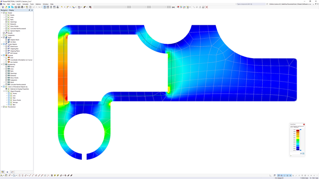
Graficzne i tabelaryczne wyświetlanie wyników dla deformacji, naprężeń i odkształceń pomaga określić bryłę gruntu. Aby to osiągnąć, skorzystaj ze specjalnych kryteriów filtrowania, które umożliwiają wybór określonych wyników.
Program na pewno cię nie zawiedzie. Jeśli chcesz graficznie ocenić wyniki w bryłach gruntu, dostępne są obiekty pomocnicze. Na przykład można zdefiniować płaszczyzny przycinania. Umożliwia to przeglądanie odpowiednich wyników na dowolnej płaszczyźnie bryły gruntu.
I nie tylko to. Wykorzystanie przekrojów wyników i brył przycinania ułatwia graficzną analizę brył gruntu.
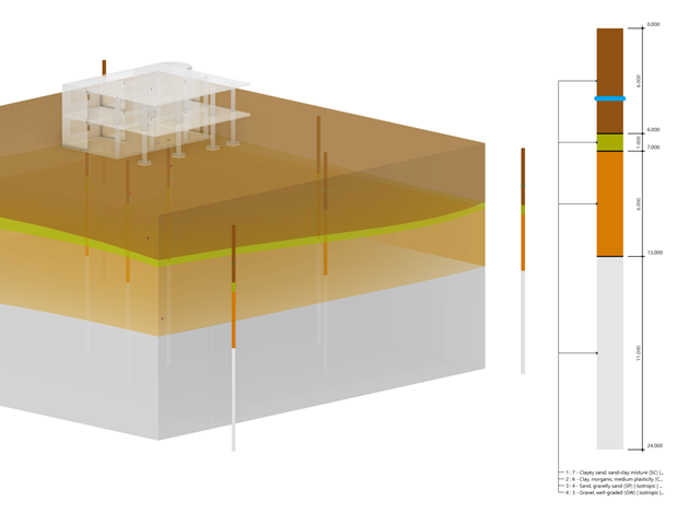
Czy wiecie, że...? Uwarstwienie gruntu, pobrane z raportów o podłożu gruntowym w miejscach wychodni, można wprowadzić bezpośrednio do programu w postaci próbek gruntu. Przypisz badane materiały gruntowe wraz z ich właściwościami do warstw.
Za pomocą danych tabelarycznych i okna dialogowego edycji można zdefiniować próbkę. Można również określić poziom wód gruntowych w próbkach gruntu.

- 002232
- Ogólne informacje
- Optymalizacja i koszty | Szacowanie emisji CO2 RFEM 6
- Optymalizacja i koszty | Szacowanie emisji CO2 RSTAB 9
Możesz być pewien, że koszty są ważnym czynnikiem w planowaniu konstrukcyjnym każdego projektu. Należy również przestrzegać przepisów dotyczących szacowania emisji. Dwuczęściowe rozszerzenie Optymalizacja i koszty/Szacowanie emisji CO2 ułatwia odnalezienie się w gąszczu norm i opcji. Wykorzystuje technologię sztucznej inteligencji (AI) optymalizacji rojem cząstek (PSO) w celu znalezienia odpowiednich parametrów dla sparametryzowanych modeli i bloków, które zagwarantują zgodność ze zwykłymi kryteriami optymalizacji. Ponadto, rozszerzenie oszacowuje koszty modelu lub emisję CO2 poprzez określenie kosztów jednostkowych lub emisji jednostkowej dla materiałów zdefiniowanych w modelu konstrukcyjnym. Dzięki temu rozszerzeniu jesteś po bezpiecznej stronie.
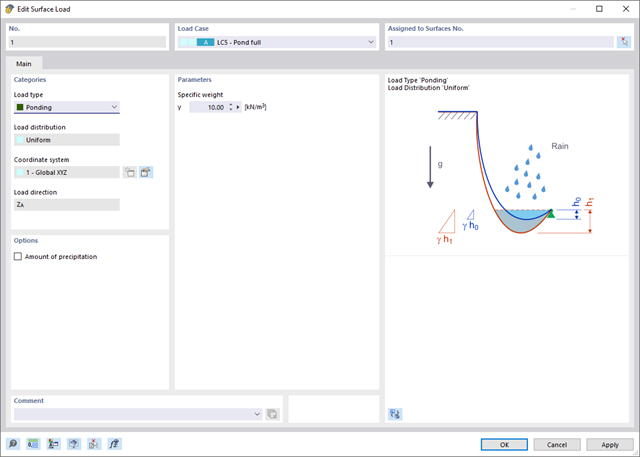
Wprowadzenie typu obciążenia Woda stojąca umożliwia symulację oddziaływań deszczu na powierzchnie wielokrotnie zakrzywione, z uwzględnieniem przemieszczeń według analizy dużych odkształceń.
Ten numeryczny proces analizy deszczowej analizuje przypisaną geometrię powierzchni i określa, które składowe wody deszczowej spływają, a które gromadzą się w postaci kałuży (kieszeni wodnych) na powierzchni. Rozmiar kałuży powoduje wówczas odpowiednie obciążenie pionowe do analizy statyczno-wytrzymałościowej.
Funkcja ta jest przeznaczona do analizy w przybliżeniu poziomych geometrii dachów membranowych pod obciążeniem deszczem.
Przejdź do filmuW porównaniu z modułem dodatkowym RF-FORM-FINDING (RFEM 5), do modułu Form-Finding dla programu RFEM 6 dodano następujące nowe funkcje:
- Określenie wszystkich warunków brzegowych dotyczących obciążenia dla analizy znajdowania kształtu (form-finding) w pojedynczym przypadku obciążenia
- Przechowywanie wyników analizy znajdowania kształtu jako stanu początkowego z możliwością późniejszego wykorzystania przy dalszej analizie modelu
- Automatyczne przypisywanie stanu początkowego z analizy znajdowania kształtu do wszystkich sytuacji obciążeniowych w sytuacji obliczeniowej za pomocą kreatorów kombinacji
- Dodatkowe geometryczne warunki brzegowe dla prętów (długość elementu nieobciążonego, maksymalny zwis w pionie, zwis w pionie w najniższym punkcie punkcie)
- Dodatkowe warunki brzegowe z uwagi na obciążenie w analizie znajdowania kształtu dla prętów (maksymalna siła w pręcie, minimalna siła w pręcie, rozciągająca składowa pozioma, rozciąganie na i-końcu, rozciąganie na końcu j, minimalne rozciąganie na końcu i, minimalne rozciąganie na końcu j)
- Typ materiału „Tkanina” i „Folia” w bibliotece materiałów
- Równoległe analizy znajdowania kształtu w jednym modelu
- Symulacja kolejnych etapów znajdowania kształtów w połączeniu z rozszerzeniem Analiza etapów konstrukcji (CSA)
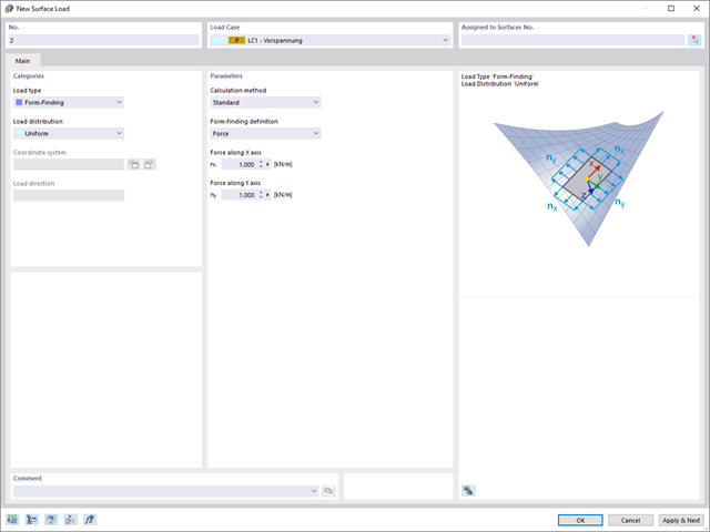
Po aktywowaniu rozszerzenia Form-Finding w Danych ogólnych, efekt znajdowania kształtu jest przypisywany do przypadków obciążeń z kategorią przypadków obciążenia "Sprężenie" w połączeniu z obciążeniami od znajdowania kształtu od pręta, powierzchni i bryły wczytaj katalog. Jest to przypadek obciążenia wstępnego naprężenia. Przekształca się on zatem w analizę znajdowania kształtu dla całego modelu ze zdefiniowanymi w nim wszystkimi elementami prętowymi, powierzchniowymi i bryłowymi. Do znajdowania kształtu odpowiednich elementów prętowych i membranowych dochodzi się w całym modelu za pomocą specjalnych obciążeń w zakresie znajdowania kształtu i regularnych definicji obciążeń. Te obciążenia znajdowania kształtu opisują oczekiwany stan odkształcenia lub siły po wyszukaniu kształtu w elementach. Obciążenia regularne opisują zewnętrzne obciążenie całego układu.
- 002458
- Ogólne informacje
- Projektowanie konstrukcji aluminiowych RFEM 6
- Projektowanie konstrukcji aluminiowych RSTAB 9
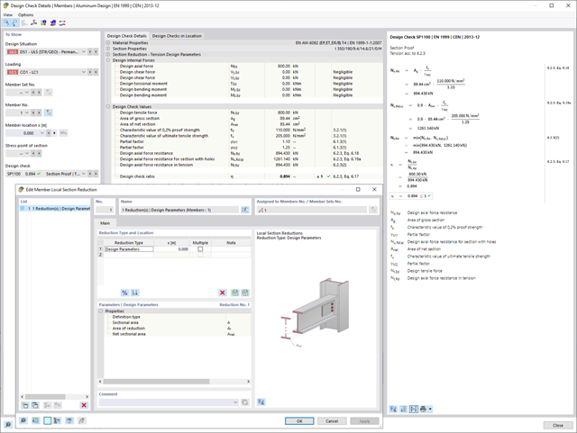
Wiesz na pewno, że podczas łączenia elementów rozciąganych za pomocą połączeń śrubowych należy wziąć pod uwagę osłabienie przekroju spowodowane otworami na śruby. Programy do analizy statyczno-wytrzymałościowej również mają na to rozwiązanie. W rozszerzeniu Aluminium Design można wprowadzić lokalną redukcję przekroju pręta. Redukcję przekroju należy wprowadzić jako wartość bezwzględną lub jako procent powierzchni całkowitej.
Wprowadzanie warstw gruntu dla potrzeb zadawania próbek gruntu odbywa się w przejrzystym oknie dialogowym. Odpowiadająca temu prezentacja graficzna zapewnia przejrzystość i ułatwia kontrolę wprowadzanych danych.
Rozszerzalna baza danych ułatwia wybór właściwości materiałowych dla gruntu. Dla realistycznego odwzorowania zachowania się materiału gruntowego można użyć modelu Mohra-Coulomba oraz model gruntu ze wzmocnieniem.
Można zdefiniować dowolną liczbę próbek i warstw gruntu. Grunt jest odwzorowany na podstawie wszystkich wprowadzonych próbek za pomocą brył 3D. Przypisanie do konstrukcji odbywa się za pomocą współrzędnych.
Zachowanie bryły gruntu jest obliczane za pomocą nieliniowej metody iteracyjnej. Obliczone naprężenia i osiadania są wyświetlane graficznie oraz w tabelach.
- 002463
- Ogólne informacje
- Projektowanie konstrukcji aluminiowych RFEM 6
- Projektowanie konstrukcji aluminiowych RSTAB 9
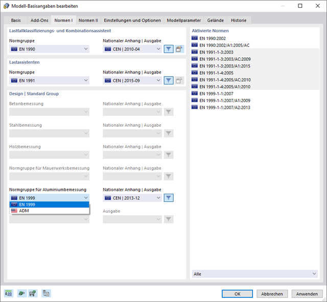
W przypadku obliczeń zgodnie z Eurokodem 9, można znaleźć parametry zintegrowanych załączników krajowych dla następujących krajów:
-
 DIN EN 1999-1-1/NA:2021-03 (Niemcy)
 -
 ÖNORM EN 1999-1-1/NA:2017-11 (Austria)
 -
 SN EN 1999-1-1/NA:2015-01 (Szwajcaria)
 -
 BDS EN 1999-1-1/NA:2014-05 (Bułgaria)
 -
 BS EN 1999-1-1/NA:2014-03 (Wielka Brytania)
 -
 CEN 1999-1-1/2013-12 (Unia Europejska)
 -
 CYS EN 1999-1-1/NA:2019-08 (Cypr)
 -
 CZE EN 1999-1-1/NA:2015-09 (Republika Czeska)
 -
 DS EN 1999-1-1/NA:2019-09 (Dania)
 -
 ELOT EN 1999-1-1/NA:2013-12 (Grecja)
 -
 EVS EN 1999-1-1/NA:2014-01 (Estonia)
 -
 HRN EN 1999-1-1/NA:2015-02 (Chorwacja)
 -
 I S. EN 1999-1-1/NA:2015-01 (Irlandia)
 -
 ILNAS EN 1999-1-1/NA:2013-12 (Luksemburg)
 -
 IST EN 1999-1-1/NA:2014-03 (Islandia)
 -
 LST EN 1999-1-1/NA:2014-03 (Litwa)
 -
 LVS EN 1999-1-1/NA:2015-01 (Łotwa)
 -
 MSZ EN 1999-1-1/NA:2014-04 (Węgry)
 -
 NBN EN 1999-1-1/NA:2014-01 (Belgia)
 -
 NEN EN 1999-1-1/NA:2014-01 (Holandia)
 -
 NF EN 1999-1-1/NA:2016-07 (Francja)
 -
 NP EN 1999-1-1/NA:2014-11 (Portugalia)
 -
 NS EN 1999-1-1/NA:2014-04 (Norwegia)
 -
 PN EN 1999-1-1/NA:2014-05 (Polska)
 -
 SFS EN 1999-1-1/NA:2018-01 (Finlandia)
 -
 SIST EN 1999-1-1/NA:2014-05 (Słowenia)
 -
 SR EN 1999-1-1/NA:2015-01 (Rumunia)
 -
 SS EN 1999-1-1/NA:2013-12 (Szwecja)
 -
 STN EN 1999-1-1/NA:2014-05 (Słowacja)
 -
 TKP EN 1999-1-1/NA:2010-01 (Białoruś)
 -
 UNE EN 1999-1-1/NA:2014-01 (Hiszpania)
 -
 UNI EN 1999-1-1/NA:2014-02 (Włochy)
- 002465
- Wyniki
- Projektowanie konstrukcji aluminiowych RFEM 6
- Projektowanie konstrukcji aluminiowych RSTAB 9
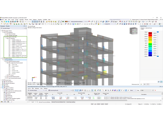
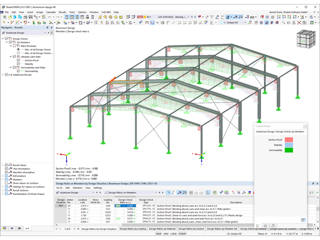
Czy projekt zakończył się sukcesem? Bardzo dobrze, teraz zaczyna się część zrelaksowana. Ponieważ program przedstawia przeprowadzone weryfikacje w formie tabelarycznej. Można wyświetlić szczegółowe informacje o wszystkich wynikach. Dzięki przejrzyście przedstawionym wzorom weryfikacyjnym można bez problemu zrozumieć wyniki. W oprogramowaniu Dlubal nie występuje efekt czarnej skrzynki.
Kontrole są przeprowadzane we wszystkich istotnych punktach prętów i wyświetlane graficznie jako profil wyników. Bardziej szczegółowe grafiki można znaleźć w wynikach wyszukiwania. Obejmuje to na przykład profil naprężenia w przekroju lub kształt drgań własnych.
Wszystkie dane wejściowe i wyniki są częścią protokołu wydruku programu RFEM/RSTAB. Dla poszczególnych obliczeń można wybrać zawartość raportu i żądaną głębokość danych wyjściowych.
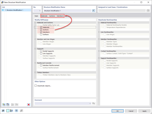
Czy wiecie, że...? W przypadkach obciążeń typu Analiza modalna można z łatwością wprowadzać zmiany konstrukcyjne. Pozwala to na przykład na indywidualne dostosowanie sztywności materiałów, przekrojów, prętów, powierzchni, przegubów i podpór. W przypadku niektórych rozszerzeń można również modyfikować sztywności. Po wybraniu obiektów ich właściwości sztywności są dostosowywane do typu obiektu. W ten sposób można je zdefiniować w osobnych zakładkach.
Czy chcesz przeanalizować uszkodzenie obiektu (na przykład słupa) w analizie modalnej? Jest to również możliwe bez żadnych problemów. Wystarczy przejść do okna Modyfikacja konstrukcji i dezaktywować odpowiednie obiekty.