AISC Steel Design Guide 26 – Design of Blast Resistant Structures [1] and in particular Example 2.1 – Preliminary Evaluation of Blast Resistance of a One-Story Structure is an ideal reference to guide engineers though a simplified blast design load application.
Idealized Blast Load Pressure-Time History
An idealized pressure-time history diagram shows how the pressure force varies over time after the explosion takes place.
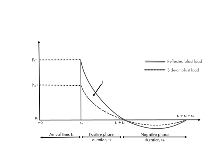
A few of the most important parameters are listed directly in the diagram, including:
- Peak overpressure (Pr or Pso) … The instantaneous pressure arriving at the structure above the ambient atmospheric pressure.
- Positive phase duration (td) … The time period for the pressure to return to ambient.
- Positive impulse (I) … The total pressure-time energy applied during the positive duration calculated by the area under the curve.
- Negative phase duration (td-) … The time period following the positive phase where the pressure falls below the atmospheric pressure.
Notice that there are two different curves represented in the idealized pressure-time history diagram, including the "side-on blast load" and the "reflected blast load" indicated by the dashed line and the solid line, respectively. The side-on blast load (also called the free-field blast load) includes the subscript "so" used commonly throughout literature. This indicates where the blast load travels parallel to a surface, rather than perpendicular. Essentially, the load will sweep over the surface with no impeding objects. An example of this includes a side wall parallel to a blast load or a rear wall with no immediate exposure to the blast.
In turn, the reflected blast load, indicated by the subscript "r", is where the blast wave strikes an angled surface other than parallel. To determine the reflected pressure, Pr, the following equation can be used.
Pr = Cr Pso
Where Pso is the side-on pressure and Cr is the reflection coefficient. Cr is a function of the angle of incidence and side-on pressure.
The image below demonstrates how the angle of incidence can be calculated when considering the initial blast wave direction and the reflected wave normal to the surface.
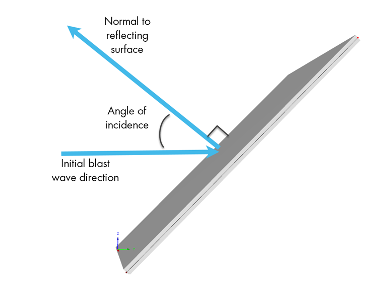
Once the angle of incidence is determined, Figure 2-193 given in the United Facilities Criteria (UFC) 3-340-02 – Structures to Resist the Effects of Accidental Explosions [2] can be used to provide the Cr value based on the Peak Incident Overpressure value.
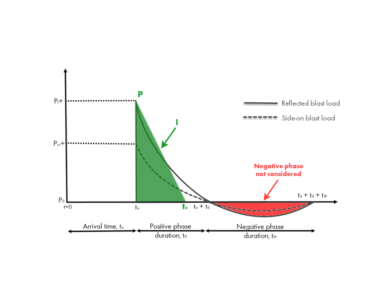
Simplified Blast Load Pressure-Time History
For design purposes, the idealized plot shown above is simplified to a triangular distribution with an instantaneous rise and linear decay under the positive phase. To maintain peak overpressure from the idealized plot as well as impulse (area under the curve), a fictitious time duration, te, is approximated as te = 2(I/P).
Extensive research to determine the relationship between charge weight, the standoff distance (distance from the structure to the explosion), and the blast parameters defined in the pressure-time plot have been carried out. Technical manuals such as resource [2] include the air blast parameters as a function of the scaled distance in the form of empirical blast parameter curves.
The negative phase is often ignored for simplification with simple structures, as there is little impact from the blast analysis. However, the negative phase becomes increasingly important when the structure's elements are weaker in the reverse loading direction or have a short fundamental period with respect to the load duration.
Additional variables that may have an influence on the blast analysis for the purposes of this article have not been taken into consideration, such as drag forces due to wind or dynamic pressures, adjacent building shielding (load reduction) and reflection (load amplification), and interior loads due to the blast wave entering the structure's openings.
AISC Design Guide 26 – Example 2.1 in RFEM
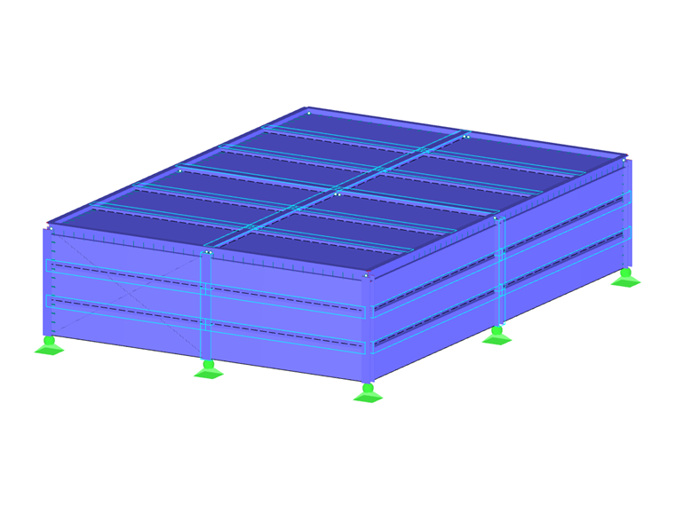
AISC Design Guide 26 – Example 2.1 [1] is an ideal reference example to apply the blast load analysis in RFEM which follows the above assumptions. The example structure is a one-story steel building with 50 ft (W) ⋅ 70 ft (L) ⋅ 15 ft (H) dimensions. In the structure's short direction, braced frames are modeled in RFEM as hot-rolled W-sections, while in the long direction, rigid frames are also modeled with W-sections. The girts and purlins are modeled with hot-rolled C-sections. The building facade includes ribbed metal panels.
The explosion has a charge weight of 500 lbs and occurs 50 ft from the front face of the structure slightly above ground elevation. With this information, the scaled distance, Z, is then calculated according to the following equation.
Front Wall
Using the scaled distance, Figure 2-15 from [2] can be utilized to directly determine the positive blast wave parameters for the reflected and side-on pressure listed below in Table 1.
| Blast Loading Parameter | From Figure 2-15 [2] | Calculated Value |
|---|---|---|
| Reflected peak pressure (+) | Pr = 79.5 psi | - |
| Side-on peak pressure (+) | Pso = 24.9 psi | - |
| Reflected impulse (+) | Ir = 31.0W1/3 | Ir = 246 psi ms |
| Side-on impulse (+) | Iso = 12.1W1/3 | Iso = 96.0 psi ms |
| Time of arrival | ta = 1.96W1/3 | ta = 15.6 ms |
| Exponential load duration (+) | td = 1.77W1/3 | td = 14.0 ms |
| Shock front velocity | U = 1.75 ft/ms | - |
Because the front wall is directly facing the initial explosion, the "reflected" variables in Table 1 are applicable to this surface. The simplified triangular approach requires the equivalent duration to be calculated to ensure the impulse (area under the curve) is preserved over the positive duration phase.
te,r = 2Ir / Pr = 2(246 psi ms) / 29.5 psi = 6.19 ms
The initial pressure-time plot is now complete for the front wall.
Side Walls and Roof
For simplicity, the scaled distance, Z, calculated for the front wall is used to determine the blast variables for the building's side walls and roof. Therefore, the side-on values in Table 1 above are used to define the pressure-time plot for this section of the building. A more detailed calculation could be carried out to consider the blast wave reduction as a function of the side wall and roof distance from the explosion.
The equivalent duration, te, is calculated using the side-on variables.
te,so = 2Iso / Pso = 2(96.0 psi ms) / 24.9 psi = 7.71 ms
Rear Wall
The scaled distance, Z, for the rear wall is modified to consider the additional length of the building. The distance is now 50 ft + 70 ft for a total of 120 ft. Therefore, Z is calculated as the following.
Figure 2-15 from [2] can be utilized again to determine the positive blast wave parameters for the side-on pressure listed below in Table 2.
| Blast Loading Parameter | From Figure 2-15 [1] | Calculated Value |
|---|---|---|
| Side-on peak pressure (+) | Pso = 4.60 psi | - |
| Side-on impulse (+) | Iso = 5.54W1/3 | Iso = 44.0 psi ms |
| Time of arrival | ta = 8.32W1/3 | ta = 66.0 ms |
| Exponential load duration (+) | td = 3.11W1/3 | td = 24.7 ms |
| Shock front velocity | U = 1.26 ft/ms | - |
The rear wall equivalent duration, te, can be calculated with the relevant variables above.
te,so = 2Iso / Pso = 2(44.0 psi ms) / 4.60 psi = 19.1 ms
Because the rear wall height is 15 ft above the ground elevation where the blast is taking place, an instantaneous rise in pressure does not occur. Rather, the velocity of the blast wave, the rear wall height, and the time of arrival are used to calculate the time to peak pressure, t².
t2 = L1 / U + ta = 15.0 ft / 1.26 ft/ms + 66.0 ms = 77.9 ms
The time to the end of the blast load, tf, can now be determined.
tf = t2 + te,so = 77.9 ms + 19.1 ms = 97.0 ms
Combining all rear wall variables calculated above, the pressure-time plot for this section of the building is complete.
Blast Load Summary
The front, side/roof, and rear walls can be compiled together to display the total pressure versus time and illustrate how the blast wave will impact the different areas of the structure over time.
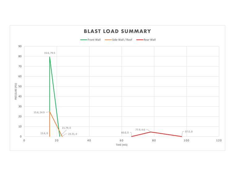
This information can now be taken into the RFEM and the RF-DYNAM Pro-Forced Vibrations add-on modules for the time diagram definitions.
Application in RFEM
Now that the pressure-time diagrams have been defined for the various sections of the building, this information can be taken into the RF-DYNAM Pro-Forced Vibrations add-on module in RFEM.
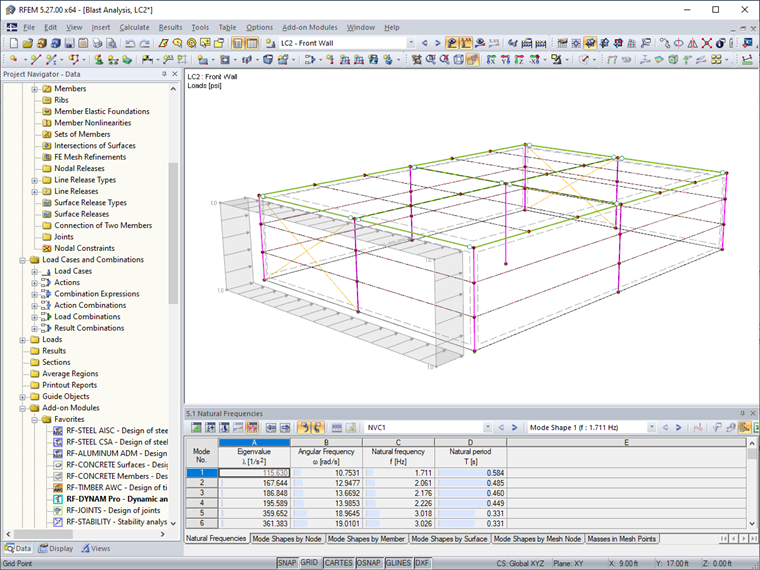
RF-DYNAM Pro-Natural Vibrations to determine the structure's natural periods, frequencies, and mode shapes is required before running the time-history analysis. This portion of the analysis is not discussed in detail for the purposes of this article.
For the time-history analysis, a general area load is applied as three separate load cases in RFEM to emulate the blast load location on the structure including LC1 – Front Wall, LC2 – Side Wall/Roof, and LC3 – Rear Wall. A magnitude of 1 kip/ft2 is used only as a placeholder, as this value will later be dependent on the time-history function.
In RF-DYNAM Pro-Forced Vibrations, the time diagrams are defined for each region of the structure.
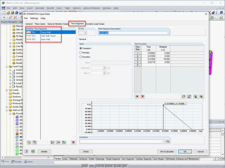
Notice that each time diagram reflects the information determined above, such as the peak pressure and equivalent duration for the front wall, side walls/roof, and rear wall.
Once the time diagrams are defined; the general area loads in RFEM are directly linked to the relevant diagram.
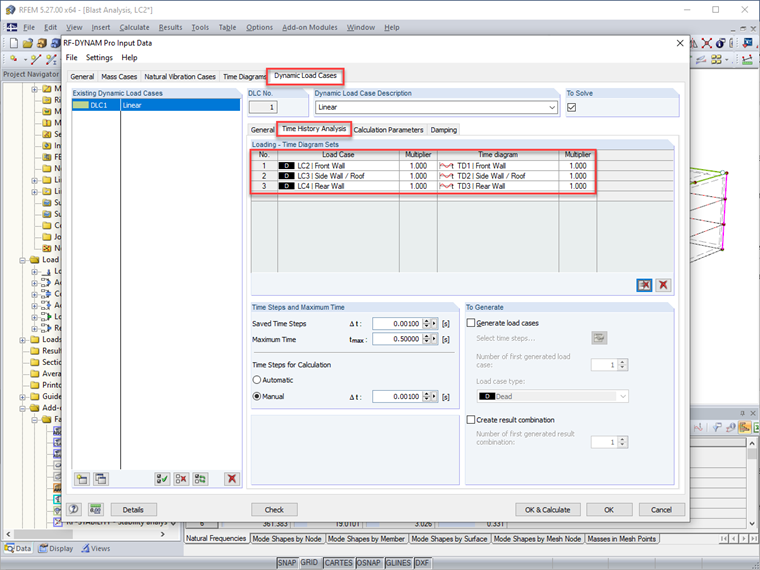
Additional variables must also be set in the add-on module before running the analysis, such as the linear implicit Newmark analysis solver, a maximum time of 0.5 seconds for the time-history analysis duration, and a time step of 0.001 seconds to be used in the calculation. Additionally, utilizing the angular frequency from the two dominant modes calculated with the natural frequency analysis along with a Lehr's damping ratio of 2%, the Rayleigh damping coefficients a and β are also set in the module.
All relevant information is now defined for the blast time-history analysis, and the RFEM and RF-DYNAM Pro calculation can be run. Evaluation tools such as the time-course monitor in RFEM can be used to assess the structure's response and safety over the course of the blast explosion. For a detailed demonstration of AISC Design Guide 26 Example 2.1 [1] in RFEM, refer to the previously recorded webinar Blast Time History Analysis in RFEM.