Nonlinear Deformation Analysis of Two-Span Beam Considering Creep

1. Input Data

Geometry

• Structural System:

System: Two-span beam
Span 1: l₁ = 5.0 m
Span 2: l₂ = 4.0 m

• Cross-Section Dimensions:

Width: b = 1000 mm
Height: h = 160 mm

• Design Properties:
  • Concrete cover c_nom = 22.0 mm
  • Existing longitudinal reinforcement: The reinforcement is arranged symmetrically in the cross-section at the top and bottom. At the top and bottom, there are 22 members with a diameter of 6.0 mm each (A_s,side = 6.22 cm²).

Loading

The two spans are subject to a permanent load, and each span is additionally subjected to a variable load:

• LC1: Load case Dead Load: g_k = 1.6 kN/m
• LC2: Load case Live Load in Span 1: q_1,k = 5.0 kN/m
• LC3: Load case Live Load in Span 2: q_2,k = 5.0 kN/m

Only the quasi-permanent design situation is governing for the deformation analysis. This results in the following three load combinations:

• CO1 = LC1 + 0.60 × LC2
• CO2 = LC1 + 0.60 × LC2 + 0.60 × LC2
• CO3 = LC1 + 0.60 × LC3

Materials

Concrete of class C20/25 and reinforcing steel of class B500S(A) are initially taken from the material library. For the Concrete material type, the Anisotropic | Damage nonlinear material model is well-suited for the deformation analysis. For the Reinforcing Steel material type, the suitable Isotropic | Plastic nonlinear material model shoul be selected.

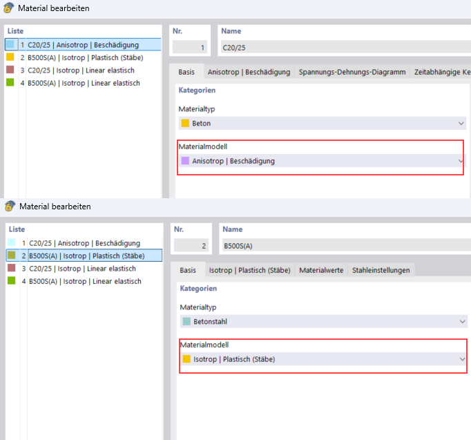
• Concrete C20/25

Once the material model is set, the specific "Anisotropic | Damage" tab appears:
Diagram Definition: For this example, a deformation calculation should be performed; therefore, the "SLS | (Mean) Values for Deflection" diagram can be used.

Compression Area:
For nonlinear analysis, the compression area is represented with the "Parabola" diagram type (according to 3.1.5) and the compressive strength f_cm.

Tension Stiffening:
For tension stiffening, the approach using the concrete residual tensile strength (Quast | Concrete) is selected.

A parabolic-rectangle diagram curve is defined in the tension area. Before cracking, the curve follows a parabolic shape where the concrete fully participates. The calculated tensile strength of concrete f_ct,R upon initial cracking is assumed to be \( f_{ct,R} = k \cdot f_{ct} = 0.6 \cdot 2.200 = 1.320~\text{N/mm}^2 \) (with a calculated cracking strain ε_cr,R of 0.1‰). Once this calculated cracking strain is exceeded, the concrete tensile strength decreases, and the stress-strain curve flattens out.

The tensile strength of concrete f_ct,R is not a constant value, but depends on the strain of the governing reinforcing steel fiber in the structural component. It decreases linearly when the crack strain ε_cr,R is exceeded and completely decreases to zero once the yield strain ε_s of the reinforcing steel is reached.

This dependency between the concrete tensile strength and steel strain is described by the factor VMB. For the range ε > ε_cr,R, the stress-strain diagram in the tension area can be described with the following equation: \( \sigma_c = VMB \cdot f_{ct,R} \)

Before cracking (ε_s < ε_cr), the reduction factor VMB remains 1.0, which means that the concrete retains its full contribution in the tension area, and the tensile strength is not reduced. There is no reduction in contribution, as the concrete has not yet cracked. After reaching the crack strain (ε_cr), the concrete begins to lose its tension stiffening. The reduction factor VMB decreases. Depending on the distribution exponent n_vmb, the reduction proceeds differently:
n_vmb = 1.0: Linear reduction.
n_vmb = 2.0: Faster, steeper reduction.
Once the yield strength of the reinforcing steel is reached, the reinforcement takes over the entire tensile stress and the concrete no longer contributes to tension stiffening. The reduction factor VMB reaches 0.

• Reinforcing Steel B500S(A)

For the reinforcing steel, the diagram type can also be set in the specific tab. In this example, the standard diagram type is used.

• Creep and Shrinkage:

Creep is initially activated in the concrete material in the Time-Dependent Properties of Concrete tab. The specific settings for creep are then stored in the Advanced Time-Dependent Properties of Concrete tab:

Shrinkage is not further analyzed: Due to the nearly symmetrical reinforcement in Span 1 and only a small reinforcement difference in Span 2, shrinkage curvatures contribute insignificantly to the total deformation. Therefore, shrinkage is deactivated.

Static Analysis Settings

The following settings are used for nonlinear deformation analysis:

• Type of Analysis: The creep is represented linearly by a modified stress-strain diagram. The strain values of the concrete are multiplied by the factor (1 + φ_ef). The "Static Analysis | Creep and Shrinkage (Linear)" analysis type should be used.
• Structure Modification: To include reinforcement stiffness already in the analysis, it is necessary to activate the member reinforcement using a structure modification for reinforced concrete.
• Creep Loading Times: You can define the loading times in the "Times" section.

FE Mesh Settings

The target element length of the finite elements was set to 100 mm. Furthermore, the cross-section FE mesh for the nonlinear analysis is provided with an offset factor of 0.50, resulting in a finer FE mesh in the cross-section, which allows for a more accurate calculation of the stress state.

2. Results

The deformation from the nonlinear calculation, considering the creep effect, results in a deflection of 18.2 mm in Span 1 at the location x=2.20m.

The representation of the basic stresses σ_x along the member illustrates that the tensile stress in Span 1 and in the column area reaches a maximum value of 1.247 N/mm².

The stress distribution in the cross-section at the location x=2.20m is illustrated by a section:

Comparison with Results of Concrete Design Add-on

A calculation of the deformation with the Concrete Design Add-on results in a deflection of 25.6 mm at the location x = 2.20 m.

A closer look at the calculation in the add-on shows that the stresses from the short-term load (without the influence of creep) are governing for determining the damage using the distribution coefficient ζ:

The “Consider initial state” function can be used to take into account the effects of short-term loading in the nonlinear calculation. First, a load combination is created that does not consider creep. This load combination is then transferred into the main load combination as an initial state:

With these settings, a deflection of 22.3 mm is obtained.

• Deformation analysis for the quasi-permanent design situation with crack state based on the corresponding loads of the SLS design situation

For the calculation of the deformation in the quasi-permanent design situation, it is possible to consider the governing crack state from the corresponding load combinations (quasi-permanent CO, frequent CO). Further information can be found in the following Knowledge Base article.

This is the case, for example, if the frequent or characteristic load combination is governing in the short term at the beginning of the service life and the quasi-permanent action acts in the further distribution until the end of the service life.

This can be easily set in the Concrete Design add-on by activating the corresponding option in the serviceability configuration.

In this example, the damage from the quasi-permanent load combination is governing for the calculation of the deformation in the characteristic load combination. The maximum deflection of the characteristic load combination in the Concrete Design add-on is 30.6 mm:

The "Consider initial state" option from another load combination is used again to consider the damage of the characteristic load combination:

This results in a deflection of 25.6 mm:

3. Comparison of Results

Load Situation	Nonlinear Analysis (NL)	Concrete Design Add-on	Ratio (NL / Add-on)
Considering damage from short-term loading	22.3	25.6	0.87
Considering damage from characteristic action	25.6	30.6	0.84

The difference between the nonlinear analysis and the use of equivalent stiffnesses in the Concrete Design add-on can be explained as follows: The add-on uses a linear-elastic material and performs the calculation analytically over the entire cross-section. The damage is taken into account by a global distribution coefficient, which means that the results tend to be conservative. In contrast, the nonlinear calculation is based on an FE model with a nonlinear concrete material model. Here, the damage is determined individually for each element of the cross-section, and effects like tension stiffening can be considered locally. As a result, crack formation and stress distribution are modeled much closer to reality.

4. Final Remarks

The nonlinear deformation analysis of a two-span reinforced concrete beam considering creep clearly shows the differences to classical linear approaches in the Concrete Design add-on. The nonlinear analysis allows for modeling the stress distribution in the cross-section close to reality, especially in the tensile area after cracking, and considers the influence of tension stiffening locally for each element in the cross-section. At the same time, the Concrete Design add-on shows a reliable, simple, and particularly convenient approach: It allows for considering the effects from short-term loads as well as the effects from permanent loads in the characteristic (and also frequent) design situations.