
If there is a load case or load combination in the program, the stability calculation is activated. You can define another load case in order to consider initial prestress, for example.
For this, you need to specify whether to perform a linear or nonlinear analysis. Depending on the case of application, you can select a direct calculation method, such as the Lanczos method or the ICG iteration method. Members not integrated in surfaces are usually displayed as member elements with two FE nodes. With such elements, the program cannot determine the local buckling of single members. That's why you have the option to divide members automatically.

You can select several methods that are available for the eigenvalue analysis:
- Direct Methods
- The direct methods (Lanczos [RFEM], roots of characteristic polynomial [RFEM], subspace iteration method [RFEM/RSTAB], and shifted inverse iteration [RSTAB]) are suitable for small to medium-sized models. You should only use these fast solver methods if your computer has a larger amount of memory (RAM).
- ICG Iteration Method (Incomplete Conjugate Gradient [RFEM])
- In contrast, this method only requires a small amount of memory. Eigenvalues are determined one after the other. It can be used to calculate large structural systems with few eigenvalues.
Use the Structure Stability add-on to perform a nonlinear stability analysis using the incremental method. This analysis delivers close-to-reality results also for nonlinear structures. The critical load factor is determined by gradually increasing the loads of the underlying load case until the instability is reached. The load increment takes into account nonlinearities such as failing members, supports and foundations, and material nonlinearities. After increasing the load, you can optionally perform a linear stability analysis on the last stable state in order to determine the stability mode.

As the first results, the program presents you with the critical load factors. You can then perform an evaluation of stability risks. For member models, the resulting effective lengths and critical loads of the members are displayed to you in tables.
Use the next result window to check the normalized eigenvalues sorted by node, member, and surface. The eigenvalue graphic allows you to evaluate the buckling behavior. This makes it easier for you to take countermeasures.

- Calculation of models consisting of member, shell, and solid elements
- Nonlinear stability analysis
- Optional consideration of axial forces from initial prestress
- Four equation solvers for an efficient calculation of various structural models
- Optional consideration of stiffness modifications in RFEM/RSTAB
- Determination of a stability mode greater than the user-defined load increment factor (Shift method)
- Optional determination of the mode shapes of unstable models (to identify the cause of instability)
- Visualization of the stability mode
- Basis for determining imperfection

- General stress analysis
- Automatic import of internal forces from RFEM/RSTAB
- Graphical and numerical output of stresses, strains, clearance, and design ratios fully integrated in RFEM/RSTAB
- User-defined specification of the limit stress
- Summary of similar structural components for the design
- Wide range of customization options for graphical output
- Clearly arranged result tables for a quick overview after the design
- Simple traceability of the results due to the complete documentation of the calculation method including all formulas
- High productivity due to the minimal amount of input data required
- Flexibility due to detailed setting options for basis and extent of calculations
- Gray zone display for unimportant value ranges (see Product Feature)

- Cross-section optimization
- Transfer of optimized sections to RFEM/RSTAB
- Design of any thin-walled section from RSECTION
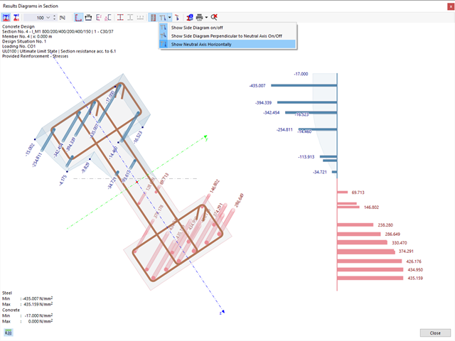
- Representation of a stress diagram on a section
- Determination of normal, shear, and equivalent stresses
- Output of stress components for the individual member internal force types
- Detailed representation of stresses in all stress points
- Determination of the largest Δσ for each stress point (for example, for fatigue design)
- Colored display of stresses and design ratios for a quick overview of the critical or oversized zones
- Output of parts lists

- Determination of principal and basic stresses, membrane and shear stresses, as well as equivalent stresses and equivalent membrane stresses
- Stress analysis for structural surfaces including simple or complex shapes
- Equivalent stresses calculated according to different approaches:
- Shape modification hypothesis (von Mises)
- Shear stress hypothesis (Tresca)
- Normal stress hypothesis (Rankine)
- Principal strain hypothesis (Bach)
- Optional optimization of surface thicknesses and data transfer to RFEM
- Output of strains
- Detailed results of individual stress components and ratios in tables and graphics
- Filter function for solids, surfaces, lines, and nodes in tables
- Transversal shear stresses according to Mindlin, Kirchhoff, or user-defined specifications
- Stress evaluation for welds at connection lines between surfaces (see the Product Feature)

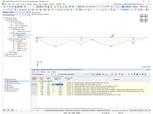
After you have completed the design, the program takes care of clearly arranged results. Thus, the program shows you the resulting maximum stresses and stress ratios sorted by section, member/surface, solid, member set, x-location, and so on. In addition to the tabular result values, the add-on shows you the corresponding cross-section graphic with stress points, stress diagram, and values as well. You can relate the design ratio to any kind of stress type. The current location is highlighted in the RFEM/RSTAB model.
In addition to the tabular evaluation, the program offers you even more. You can also graphically check the stresses and design ratios on the RFEM/RSTAB model. It is possible for you to adjust the colors and values individually.
The display of result diagrams of a member or set of members enables you a targeted evaluation. For each design location, you can open the respective dialog box to check the design-relevant section properties and stress components of any stress point. Finally, you have the option of printing the corresponding graphic, including all design details.

- Consideration and display of story masses
- Listing of structural elements and their information
- Automated creation of result sections on shear walls
- Output of section resultants in global direction for determining shear forces
- Optional definition of rigid diaphragm by story (story modeling)
- Stiffness type Floor Slab - Rigid Diaphragm
- Defining floor sets,
- for example, calculation of slabs as a 2D position within the 3D model
- Shear walls: Automatic definition of result members with any cross-section
- Design of rectangular cross-sections using the Concrete Design add-on
- Definition of deep beams
- Design with the Concrete Design add-on
- Tabular output of story actions, interstory drift, and center points of mass and stiffness, as well as the forces in shear walls
- Separate result display of the floor and stiffening design
- Optional neglecting of openings of a certain size
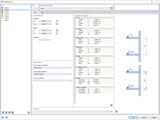
You have two options for a building model. You can create it when you start modeling the structure, or activate it afterwards. In the building model, you can then directly define the stories and manipulate them.
When manipulating the stories, you can choose whether to modify or retain the included structural elements using various options.
RFEM does some of the work for you. For example, it automatically generates result sections, so you don't need to perform a lot of calculations.

You can display the results as usual via the Results navigator. Furthermore, the dialog box of the add-on shows you the information about the individual floors. Thus, you always have a good overview.

- Artificial intelligence technology (AI): Particle swarm optimization (PSO)
- Structure optimization according to the minimum weight or deformation
- Use of any number of optimization parameters
- Specification of variable ranges
- Optimization of cross-sections and materials
- Parameter definition types
- Optimization | Ascending or Optimization | Descending
- Application of parametric models and blocks
- Code-based JavaScript parametrization of blocks
- Optimization taking into account the design results
- Tabular display of the best model mutations
- Real-time display of the model mutations in the optimization process
- Model cost estimation by specifying unit prices
- Determination of the global warming potential GWP when realizing the model by estimating the CO2 equivalent
- Specification of weight-, volume-, and area-based units (price and CO2e)

Did you know? The structural optimization in the programs RFEM and RSTAB is a completion of the parametric input. It is a parallel process beside the actual model calculation with all its regular calculation and design definitions. The add-on assumes that your model or block is built with a parametric context and is controlled in its entirety by global control parameters of the "optimization" type. Therefore, these control parameters have a lower and upper limit and a step size to delimit the optimization range. If you want to find optimal values for the control parameters, you have to specify an optimization criterion (for example, minimum weight) with the selection of an optimization method (for example, particle swarm optimization).
You can already find the cost and CO2 emission estimation in the material definitions. You can activate both options individually in each material definition. The estimation is based on a unit for unit cost or unit emission for members, surfaces, and solids. In this case, you can select whether to specify the units by weight, volume, or area.

There are two methods that you can use for the optimization process, with which you can find optimal parameter values according to a weight or deformation criterion.
The most efficient method with the littlest calculation time is the near-natural particle swarm optimization (PSO). Have you heard or read about it? This artificial intelligence (AI) technology has a strong analogy to the behavior of flocks of animals, looking for a resting place. In such swarms, you can find many individuals (cf. optimization solution - for example, weight) who like to stay in a group and follow the group movement. Let's assume that each individual swarm member has a need to rest at an optimal resting place (cf. best solution - for example, lowest weight). This need increases as the resting place is approached. Thus, the swarm behavior is also influenced by the properties of the space (cf. result diagram).
Why the excursion into biology? Quite simply – the PSO process in RFEM or RSTAB proceeds in a similar way. The calculation run starts with an optimization result from a random assignment of the parameters to be optimized. It repeatedly determines new optimization results with varied parameter values, which are based on the experience of the previously performed model mutations. The process continues until the specified number of possible model mutations is reached.
As an alternative to this method, the program also offers you a batch processing method. This method attempts to check all possible model mutations by randomly specifying the values for the optimization parameters until a predetermined number of possible model mutations is reached.
After calculating a model mutation, both variants also check the respective activated design results of the add-ons. Furthermore, they save the variant with the corresponding optimization result and value assignment of the optimization parameters if the utilization is < 1.
You can determine the estimated total costs and emission from the respective sums of the individual materials. The sums of the materials are composed of the weight-based, volume-based, and area-based partial sums of the member, surface, and solid elements.

Both optimization methods have one thing in common. At the end of the process, they provide you with a list of model mutations from the stored data. Here you can find the details of the controlling optimization result and the associated value assignment of the optimization parameters. This list is organized in descending order. You can find the assumed best solution shown in the first line. For this, the optimization result with its determined value assignment is closest to the optimization criterion. All add-on results have a utilization < 1. Furthermore, once the analysis is completed, the program will adjust the value assignment to that of the optimal solution for the optimization parameters in the global parameter list.
In the material dialog boxes, you can find the additional tabs "Cost Estimation" and "Estimation of CO2 Emissions". They show you the individual estimated sums of the assigned members, surfaces, and solids per unit weight, volume, and area. Furthermore, these tabs show the total cost and emission of all assigned materials. This gives you a good overview of your project.

Once you activate the Form-Finding add-on in the Base Data, a form-finding effect is assigned to the load cases with the load case category "Prestress" in conjunction with the form-finding loads from the member, surface, and solid load catalog. This is a prestress load case. It thus mutates into a form-finding analysis for the entire model with all member, surface, and solid elements defined in it. You reach the form-finding of the relevant member and membrane elements amid the overall model by using special form-finding loads and regular load definitions. These form-finding loads describe the expected state of deformation or force after the form-finding in the elements. The regular loads describe the external loading of the entire system.

Do you know exactly how the form-finding is performed? First, the form-finding process of the load cases with the load case category "Prestress" shifts the initial mesh geometry to an optimally balanced position by means of iterative calculation loops. For this task, the program uses the Updated Reference Strategy (URS) method by Prof. Bletzinger and Prof. Ramm. This technology is characterized by equilibrium shapes that, after the calculation, comply almost exactly with the initially specified form-finding boundary conditions (sag, force, and prestress).
In addition to the pure description of the expected forces or sags on the elements to be formed, the integral approach of the URS also enables a consideration of regular forces. In the overall process, this allows, for example, for a description of the self-weight or a pneumatic pressure by means of corresponding element loads.
All these options give the calculation kernel the potential to calculate anticlastic and synclastic forms that are in an equilibrium of forces for planar or rotationally symmetric geometries. In order to be able to realistically implement both types individually or together in one environment, the calculation provide you with two ways to describe the form-finding force vectors:
- Tension method - description of the form-finding force vectors in space for planar geometries
- Projection method - description of the form-finding force vectors on a projection plane with fixation of the horizontal position for conical geometries

The form-finding process gives you a structural model with active forces in the "prestress load case" This load case shows the displacement from the initial input position to the form-found geometry in the deformation results. In the force or stress-based results (member and surface internal forces, solid stresses, gas pressures, and so on), it clarifies the state for maintaining the found form. For the analysis of the shape geometry, the program offers you a two-dimensional contour line plot with the output of the absolute height and an inclination plot for the visualization of the slope situation.
Now, a further calculation and structural analysis of the entire model is performed. For this purpose, the program transfers the form-found geometry including the element-wise strains into a universally applicable initial state. You can now use it in the load cases and load combinations.
Compared to the RF‑/STABILITY (RFEM 5) and RSBUCK (RSTAB 8) add-on modules, the following new features have been added to the Structure Stability add-on for RFEM 6 / RSTAB 9:
- Activation as a property of a load case or a load combination
- Automated activation of the stability calculation via combination wizards for several load situations in one step
- Incremental load increase with user-defined termination criteria
- Modification of the mode shape normalization without recalculation
- Result tables with filter option
Compared to the RF-FORM-FINDING add-on module (RFEM 5), the following new features have been added to the Form-Finding add-on for RFEM 6:
- Specification of all form-finding load boundary conditions in one load case
- Storage of form-finding results as initial state for further model analysis
- Automatic assignment of the form-finding initial state via combination wizards to all load situations of a design situation
- Additional form-finding geometry boundary conditions for members (unstressed length, maximum vertical sag, low-point vertical sag)
- Additional form-finding load boundary conditions for members (maximum force in member, minimum force in member, horizontal tension component, tension at i-end, tension at j-end, minimum tension at i-end, minimum tension at j-end)
- Material types "Fabric" and "Foil" in material library
- Parallel form-findings in one model
- Simulation of sequentially building form-finding states in connection with the Construction Stages Analysis (CSA) add-on
Compared to the RF‑/STEEL add-on module (RFEM 5 / RSTAB 8), the following new features have been added to the Stress-Strain Analysis add-on for RFEM 6 / RSTAB 9:
- Treatment of members, surfaces, solids, welds (line welded joints between two and three surfaces with subsequent stress design)
- Output of stresses, stress ratios, stress ranges, and strains
- Limit stress depending on the assigned material or a user-defined input
- Individual specification of the results to be calculated through freely assignable setting types
- Non-modal result details with prepared formula display and additional result display on the cross-section level of members
- Output of the design check formulas used
Are you afraid that your project will end in the digital tower of Babel? The Building Model add-on for RFEM supports you in your work on a construction project with several stories. It allows you to define a building by means of stories at specified elevations. You can adjust the stories in many ways afterwards and also select the story slab stiffness. Information about the stories and the entire model (center of gravity, center of rigidity) is displayed for you in tables and graphics.

You can be sure that costs are an important factor in the structural planning of any project. It is also essential to adhere to the provisions on emissions estimation. The two-part add-on Optimization & Costs/CO2 Emission Estimation makes it easier for you to find your way through the jungle of standards and options. It uses the artificial intelligence technology (AI) of the particle swarm optimization (PSO) to find the right parameters for parameterized models and blocks that guarantee the compliance with the usual optimization criteria. This add-on also estimates the model costs or CO2 emissions by specifying unit costs or emissions per material definition for the structural model. With this add-on, you are on the safe side.

Reinforced concrete usually answers the question "How much can you carry?" simply with "Yes". Nevertheless, you need a three-dimensional moment-moment-axial force interaction diagram for the graphical output of the ultimate limit state of reinforced concrete cross-sections. The Dlubal structural analysis software offers you just that.
With the additional display of the load action, you can easily recognize or visualize whether the limit resistance of a reinforced concrete cross-section is exceeded. Since you can control the diagram properties, you can customize the appearance of the My-Mz-N diagram to suit your needs.

Did you know that you can also display the moment-axial force interaction diagrams (M‑N diagrams) graphically? This allows you to display the cross-section resistance in the case of an interaction of a bending moment and an axial force. In addition to the interaction diagrams related to the cross-section axes (My‑N diagram and Mz‑N diagram), you can also generate an individual moment vector to create an Mres‑N interaction diagram. You can display the section plane of the M‑N diagrams in the 3D interaction diagram. The program displays the corresponding value pairs of the ultimate limit state in a table. The table is dynamically linked to the diagram so that the selected limit point is also displayed in the diagram.

Do you want to determine the biaxial bending resistance of a reinforced concrete cross-section? For this, you have to activate a moment-moment interaction diagram (My-Mz diagram) first. This My-Mz diagram represents a horizontal section through the three-dimensional diagram for the specified axial force N. Due to the coupling to the 3D interaction diagram, you can also visualize the section plane there.
.png?mw=640&hash=5a991f211d984ac624978f514e70c53da263e5d9)
Depending on the axial force N, you can generate a moment curvature line for any moment vector. The program also shows you the value pairs of the displayed diagram in a table. Furthermore, you can activate the secant stiffness and tangent stiffness of the reinforced concrete cross-section, belonging to the moment curvature diagram, as an additional diagram.
The structural analysis program provides you with a clear overview of all performed design checks for the design standard. You have to determine a design criterion for each design check. In addition to the ultimate limit state and the serviceability limit state design, the program checks the design rules of the standard. For each design check, there are the design details including the initial values, intermediate results, and final results, arranged in a structured way. An information window in the design details shows you the calculation process with the applied formulas, standard sources, and results in great detail.
You can display the existing stresses and strains of a concrete cross-section and the reinforcement as a 3D stress image or 2D graphic. Depending on which results do you select in the result tree of the design details, the stresses or strains are displayed to you in the defined longitudinal reinforcement under the load actions or the limit internal forces.
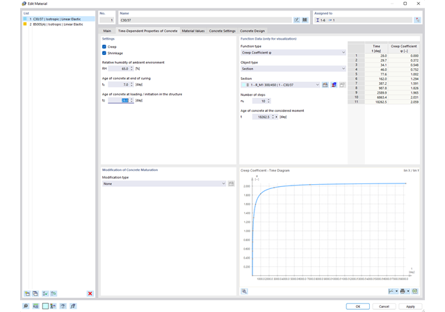
Time-dependent concrete properties, such as creep and shrinkage, are very important for your calculation. You can define them directly for the material in the structural analysis program. In the input dialog box, the time course of the creep or shrinkage function is displayed to you graphically. You can easily select the modification of the applied concrete age, for example, due to a temperature treatment.