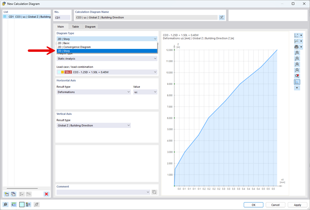
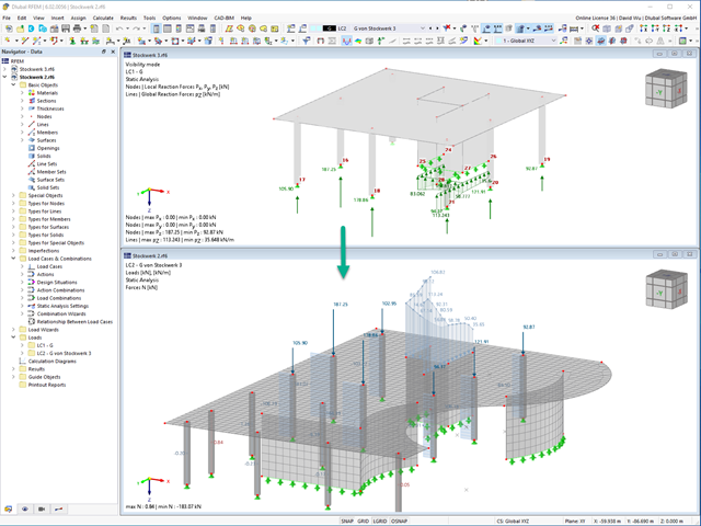
The "2D | Story" calculation diagram type is used to create result diagrams via the building axis. This allows you to easily analyze the behavior of the entire building under static and dynamic effects.
You can use this diagram type, for example, to visualize the seismic force over the building height.
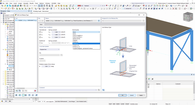
You can simulate the static friction effects between two supporting components along a line using the "Friction" nonlinearity in the Line Release Type.
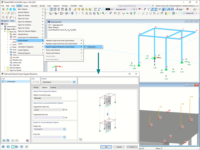
Use the "Import Support Reactions" Load Wizard in RFEM 6 and RSTAB 9 to easily transfer reaction forces from other models. The wizard allows you to connect all or several nodal and line loads of different models with each other in a few steps.
The load transfer from load cases and load combinations can be carried out automatically or manually. It's necessary that the models are saved in the same Dlubal Center project.
The "Import Support Reactions" load wizard supports the concept of positional statics and allows you to digitally connect the individual positions.
Go to Explanatory Video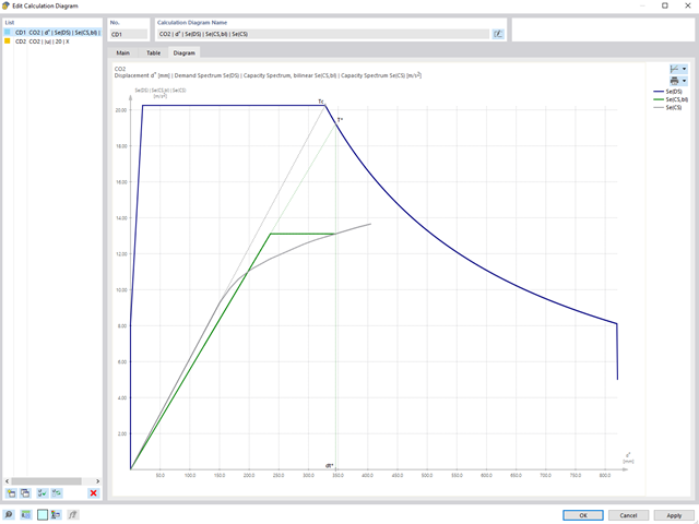
During the calculation, the selected horizontal load is increased in load steps. A static nonlinear analysis is carried out for each load step until reaching the specified limit condition.
The results of the pushover analysis are extensive. On one hand, the structure is analyzed for its deformation behavior. This can be represented by a force-deformation line of the system (a capacity curve). On the other hand, the response spectrum effect can be displayed in the ADRS display (Acceleration-Displacement Response Spectrum). The target displacement is automatically determined in the program based on these two results. The process can be evaluated graphically and in tables.
The individual acceptance criteria can then be graphically evaluated and assessed (for the next load step of the target displacement, but also for all other load steps). The results of the static analysis are also available for the individual load steps.
This function provides you with the option to adopt reaction forces from other models as nodal and line loads.
The option not only transfers the reaction load as an action, but digitally couples the support load of the original model with the load size of the target object. The subsequent changes in the original model are automatically adopted in the target model.
This technology supports the concept of positional statics and allows you to digitally connect the individual positions of the same Dlubal Center project.
Go to Explanatory Video
Do you want to consider other loads as masses in addition to the static loads? The program allows that for nodal, member, line and surface loads. For this, you need to select the Mass load type when defining the load of interest. Define a mass or mass components in the X, Y, and Z directions for such loads. For nodal masses, you have an additional option to also specify moments of inertia X, Y, and Z in order to model more complex mass points.

You can already see it in the image: Imperfections can also be taken into account when defining a modal analysis load case. The imperfection types that you can use in the modal analysis are notional loads from load case, initial sway via table, static deformation, buckling mode, dynamic mode shape, and group of imperfection cases.

- Calculation of stationary incompressible turbulent wind flow using the SimpleFOAM solver from the OpenFOAM® software package
- Numerical scheme according to the first and second order
- Turbulence models RAS k-ω and RAS k-ε
- Consideration of surface roughness depending on model zones
- Model design via VTP, STL, OBJ, and IFC files
- Operation via bidirectional interface of RFEM or RSTAB for importing model geometries with standard-based wind loads and exporting wind load cases with probe-based printout report tables
- Intuitive model changes via drag & drop and graphical adjustment assistance
- Generation of a shrink-wrap mesh envelope around the model geometry
- Consideration of environmental objects (buildings, terrain, and so on)
- Height-dependent description of the wind load (wind speed and turbulence intensity)
- Automatic meshing depending on a selected depth of detail
- Consideration of layer meshes near the model surfaces
- Parallelized calculation with optimal utilization of all processor cores of a computer
- Graphical output of the surface results on the model surfaces (surface pressure, Cp coefficients)
- Graphical output of the flow field and vector results (pressure field, velocity field, turbulence – k-ω field, and turbulence – k-ε field, velocity vectors) on Clipper/Slicer planes
- Display of 3D wind flow via animated streamline graphics
- Definition of point and line probes
- Multilingual user interface (German, English, Czech, Spanish, French, Italian, Polish, Portuguese, Russian, and Chinese)
- Calculations of several models in one batch process
- Generator for creating rotated models to simulate different wind directions
- Optional interruption and continuation of the calculation
- Individual color panel per result graphic
- Display of diagrams with separate output of results on both sides of a surface
- Output of the dimensionless wall distance y+ in the mesh inspector details for the simplified model mesh
- Determination of the shear stress on the model surface from the flow around the model
- Calculation with an alternative convergence criterion (you can select between the residual types pressure or flow resistance in the simulation parameters)
By solving the numerical flow problem, you can obtain the following results on and around the model:
- Pressure on structure surface
- Coefficient Cp distribution on the structure surfaces
- Pressure field about the structure geometry
- Velocity field about the structure geometry
- Turbulence k-ω field about the structure geometry
- Turbulence k-ε field about the structure geometry
- Velocity vectors about the structure geometry
- Streamlines about the structure geometry
- Forces on member-shaped structures that were originally generated from member elements
- Convergence diagram
- Direction and size of the flow resistance of the defined structures
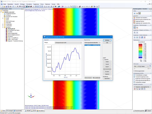
Despite this amount of information, RWIND 2 remains clearly arranged, as is typical for the Dlubal programs. You can specify freely definable zones for a graphic evaluation. Voluminously displayed flow results about the structure geometry are often confusing – you know the problem for sure. That's why RWIND Basic provides freely movable section planes for the separate display of the "solid results" in a plane. For the 3D branched streamline result, you have an option to select between a static and an animated display in the form of moving line segments or particles. This option helps you to represent the wind flow as a dynamic effect.
You can export all results as a picture or, especially for the animated results, as a video.
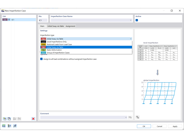
The organization of imperfections is efficiently solved by imperfection cases. The cases allow you to describe an imperfection from local imperfections, equivalent loads, initial sway via table (new), a static deformation, a buckling mode, a dynamic mode shape, or a combination of all these types (new).
Go to Explanatory Video
Compared to the RF‑SOILIN add-on module (RFEM‑5), the following new features have been added to the Geotechnical Analysis add-on for RFEM 6:
- Creation of the layered soil as a 3D model from the entirety of the defined soil samples
- Recognized material law according to Mohr-Coulomb for soil simulation
- Graphical and tabular output of stresses and strains at any depth of the soil
- Optimal consideration of the soil-structure interaction on the basis of an overall model

Did you know that Equivalent static loads are generated separately for each relevant eigenvalue and excitation direction. These loads are saved in a load case of the Response Spectrum Analysis type and RFEM/RSTAB performs a linear static analysis.
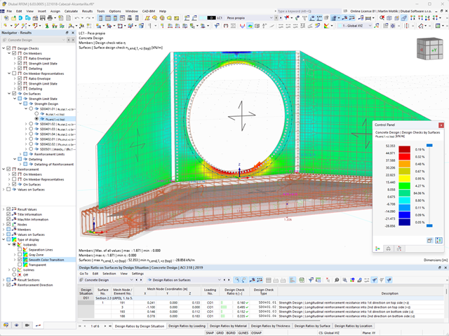
The standards already specify the approximation methods (for example, deformation calculation according to EN 1992‑1‑1, 7.4.3, or ACI 318‑19, 24.3.2.5) that you need for your deformation calculation. In this case, the so-called effective stiffnesses are calculated in the finite elements in accordance with the existing limit state with / without cracks. You can then use these effective stiffnesses to determine the deformations by means of another FEM calculation.
Consider a reinforced concrete cross-section for the calculation of the effective stiffnesses of the finite elements. Based on the internal forces determined for the serviceability limit state in RFEM, you can classify the reinforced concrete cross-section as "cracked" or "uncracked". Do you consider the effect of the concrete between the cracks? In this case, this is done by means of a distribution coefficient (for example, according to EN 1992‑1‑1, Eq. 7.19, or ACI 318‑19, 24.3.2.5). You can assume the material behavior for the concrete to be linear-elastic in the compression and tension zone until reaching the concrete tensile strength. This procedure is sufficiently precise for the serviceability limit state.
When determining the effective stiffnesses, you can take into accout the creep and shrinkage at the "cross-section level." You don't need to consider the influence of shrinkage and creep in statically indeterminate systems in this approximation method (for example, tensile forces from shrinkage strain in systems restrained on all sides are not determined and have to be considered separately). In summary, the deformation calculation is carried out in two steps:
- Calculation of effective stiffnesses of the reinforced concrete cross-section assuming linear-elastic conditions
- Calculation of the deformation using the effective stiffnesses with FEM
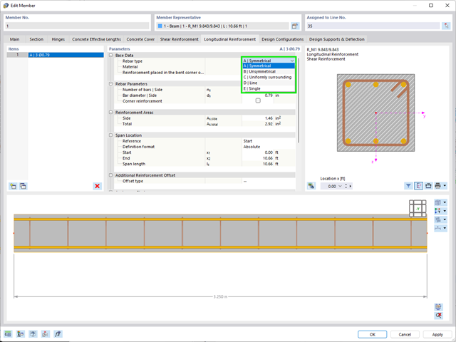
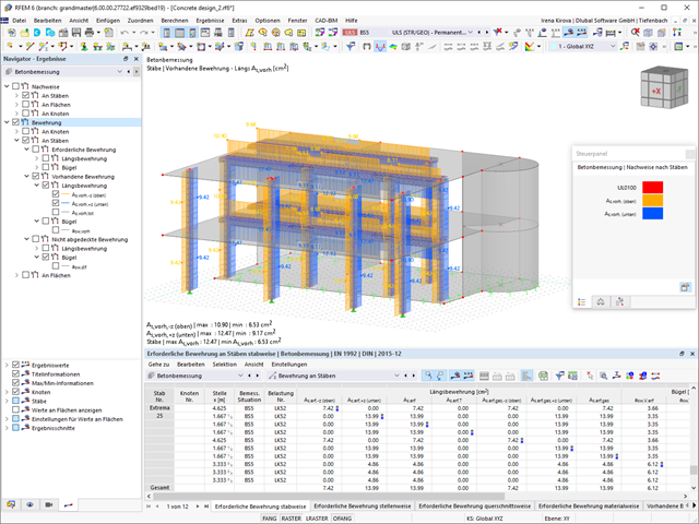
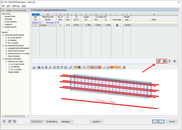
- Determination of longitudinal, shear, and torsional reinforcement
- Representation of minimum and compression reinforcement
- Determination of neutral axis depth, concrete and steel strains
- Design of member sections affected by bending about two axes
- Design of tapered members
- Design of RSECTION cross-sections (see this Product Feature)
- Determination of deformation in state II; for example, according to EN 1992‑1‑1, 7.4.3, and ACI 318‑19 24.2.3, Table 24.2.3.5
- Considering tension stiffening
- Considering creep and shrinkage
- Fatigue design according to EN 1992‑1‑1, Section 6.8 (see this Product Feature)
- Simplified fire resistance design according to EN 1992‑1‑2 for Columns (Section 5.3.2) and Beams (Section 5.6) (see this Product Feature)
- Seismic design according to EC 8 (see this Product Feature)
- Precise breakdown of reasons for failed design
- Design details of all design locations for better traceability of reinforcement determination
- Optional cross-section optimization
- Visualization of concrete section with reinforcement in 3D rendering
- Creation of 2D interaction diagrams; for example, M-N diagram
- Visualization of section resistance in 3D interaction diagram
- Output of moment-curvature diagram
- Automatic import of internal forces from RFEM/RSTAB
- Optional consideration of creep
- Automatic determination of planned and unintentional eccentricity from the second-order analysis in addition to the existing eccentricity
- Determination of internal forces according to the linear static analysis and the second-order analysis
- Analysis of governing design locations along the column due to existing loading
- Output of the required longitudinal and stirrup reinforcement
- Summary of design ratios, including all design details
- Consideration of 7 local deformation directions (ux, uy, uz, φx, φy, φz, ω) or 8 internal forces (N, Vu, Vv, Mt,pri, Mt,sec, Mu, Mv, Mω) when calculating member elements
- Usable in combination with a structural analysis according to linear static, second-order, and large deformation analysis (imperfections can also be taken into account)
- In combination with the Stability Analysis add-on, allows you to determine critical load factors and mode shapes of stability problems such as torsional buckling and lateral-torsional buckling
- Consideration of end plates and transverse stiffeners as warping springs when calculating I-sections with automatic determination and graphical display of the warping spring stiffness
- Graphical display of the cross-section warping of members in the deformation
- Full integration with RFEM and RSTAB
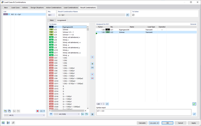
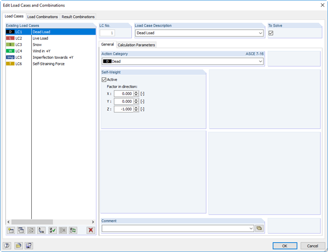
RFEM 6 offers you a wide range of helpful and efficient functions for working with load combinations. You can add the load cases included in load combinations together and then calculate them in consideration of the corresponding factors (partial safety and combination factors, coefficients regarding consequence classes, and so on). Generate the load combinations automatically in compliance with the combination expressions of the standard. You can perform the calculation according to the linear static analysis, second-order analysis, or large deformation analysis, as well as for post-critical analysis. Optionally, you can define whether the internal forces should be related to the deformed or non-deformed structure.
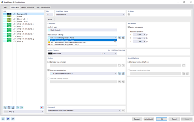
Select the individually suitable calculation parameters for your project: You can perform the calculation for all member types according to the linear static, second-order, or large deformation analysis. You have this selection option for load cases and load combinations. You can specifically set further calculation parameters for load cases, load combinations, and result combinations, which ensures a high degree of flexibility with regard to the calculation method and detailed specifications.
- 3D incompressible wind flow analysis with OpenFOAM® software package
- Direct model import from RFEM or RSTAB including neighboring and terrain models (3DS, IFC, STEP files)
- Model design via STL or VTP files independent of RFEM or RSTAB
- Simple model changes using Drag and Drop and graphical adjustment assistance
- Automatic corrections of the model topology with shrink wrap networks
- Option to add objects from the environment (buildings, terrain ...)
- Wind load determined over the height of the building, depending on standard-specific parameters (velocity, turbulence intensity)
- K-epsilon and K-omega turbulence models
- Automatic mesh generation adjusted to the selected depth of detail
- Parallel calculation with optimal utilization of the capacity of multicore computers
- Results in just minutes for low-resolution simulations (up to 1 million cells)
- Results within a few hours for simulations with medium/high resolution (1‑10 million cells)
- Graphical display of results on the Clipper/Slicer planes (scalar and vector fields)
- Graphical display of streamlines
- Streamline animation (optional video creation)
- Definition of point and line probes
- Display of aerodynamic pressure coefficients
- Graphical display of turbulence properties in the wind field
- Optional meshing using the boundary layer option for the area near the model surface
- Consideration of rough model surfaces possible
- Optional use of a seond-order numerical Order
- Multilingual user interface (for example, German, English, Spanish, French)
- Documentation possible in the RFEM and RSTAB printout report
Always keep an eye on your results. In addition to the resulting load cases in RFEM or RSTAB (see below), the results from the aerodynamics analysis in RWIND 2 represent the flow problem as a whole:
- Pressure on structure surface
- Pressure field about structure geometry
- Velocity field about structure geometry
- Velocity vectors about structure geometry
- Flow lines about structure geometry
- Forces on member-shaped structures that were originally generated from member elements
- Convergence diagram
- Direction and size of the flow resistance of the defined structures
These results are displayed in the RWIND 2 environment and evaluated graphically. The flow results around the structure geometry in the overall display are rather confusing, but the program has a solution for this. In order to present clearly arranged results, freely movable section planes are displayed for the separate display of the 'solid results' in a plane. Accordingly, for the 3D branched streamline result, the program presents you an animated display in the form of moving lines or particles in addition to the static one. This option helps to represent the wind flow as a dynamic effect.
You can export all results as a picture or, especially for the animated results, as a video.
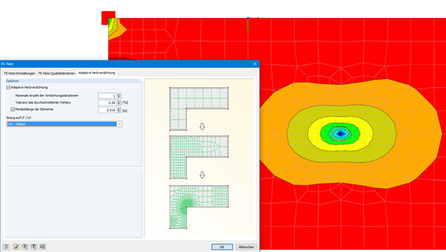
With this function, it is possible to refine the FE mesh on surfaces automatically. The mesh refinement is gradual. In each step, the FE mesh is recreated based on an error comparison of the results in the previous calculation step. The numerical error is evaluated from the results of surface elements and is based on the energy formulation of Zienkiewicz-Zhu.
The error evaluation is carried out for a linear static analysis. We select a load case (or load combination) for which the FE mesh is generated. The FE mesh is then used for all calculations.
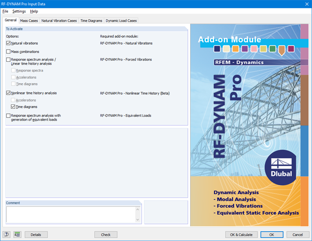
RF-/DYNAM Pro - Nonlinear Time History is integrated in the structure of RF‑/DYNAM Pro - Forced Vibrations and extended by two nonlinear analysis methods (one nonlinear analysis in RSTAB).
Force-time diagrams can be entered as transient, periodic, or as a function of time. Dynamic load cases combine the time diagrams with the static load cases, which provides high flexibility. Furthermore, it is possible to define time steps for the calculation, structural damping, and export options in the dynamic load cases.
- Full integration in RFEM/RSTAB with import of geometry and load case data
- Automatic selection of members for design according to specified criteria (e.g. only vertical members)
- In connection with the extension EC2 for RFEM/RSTAB, you can perform the design of reinforced concrete compression elements according to the method based on nominal curvature in compliance with EN 1992 -1‑1:2004 (Eurocode 2) and the following National Annexes:
-
 DIN EN 1992-1-1/NA/A1:2015-12 (Germany)
 -
 ÖNORM B 1992-1-1:2018-01 (Austria)
 -
 Belgium NBN EN 1992-1-1 ANB:2010 for design at normal temperature, and NBN EN 1992-1-2 ANB:2010 for fire resistance design (Belgium)
 -
 BDS EN 1992-1-1:2005/NA:2011 (Bulgaria)
 -
 EN 1992-1-1 DK NA:2013 (Denmark)
 -
 NF EN 1992-1-1/NA:2016-03 (France)
 -
 SFS EN 1992-1-1/NA:2007-10 (Finland)
 -
 UNI EN 1992-1-1/NA:2007-07 (Italy)
 -
 LVS EN 1992-1-1:2005/NA:2014 (Latvia)
 -
 LST EN 1992-1-1:2005/NA:2011 (Lithuania)
 -
 MS EN 1992-1-1:2010 (Malaysia)
 -
 NEN-EN 1992-1-1+C2:2011/NB:2016 (Netherlands)
 -
 NS EN 1992-1 -1:2004-NA:2008 (Norway)
 -
 PN EN 1992-1-1/NA:2010 (Poland)
 -
 NP EN 1992-1-1/NA:2010-02 (Portugal)
 -
 SR EN 1992-1-1:2004/NA:2008 (Romania)
 -
 SS EN 1992-1-1/NA:2008 (Sweden)
 -
 SS EN 1992-1-1/NA:2008-06 (Singapore)
 -
 STN EN 1992-1-1/NA:2008-06 (Slovakia)
 -
 SIST EN 1992-1-1:2005/A101:2006 (Slovenia)
 -
 UNE EN 1992-1-1/NA:2013 (Spain)
 -
 CSN EN 1992-1-1/NA:2016-05 (Czech Republic)
 -
 BS EN 1992-1-1:2004/NA:2005 (United Kingdom)
 -
 TKP EN 1992-1-1:2009 (Belarus)
 -
 CYS EN 1992-1-1:2004/NA:2009 (Cyprus)
-
- In addition to the National Annexes (NA) listed above, you can define a specific NA, applying user-defined limit values and parameters.
- Optional consideration of creep
- Diagram-based determination of buckling lengths and slenderness from the restraint ratios of columns
- Automatic determination of ordinary and unintentional eccentricity from additionally available eccentricity according to the second-order analysis
- Design of monolithic structures and precast elements
- Analysis with regard to the standard reinforced concrete design
- Determination of internal forces according to the linear static analysis and the second-order analysis
- Analysis of governing design locations along the column due to existing loading
- Output of required longitudinal and stirrup reinforcement
- Fire resistance design according to the simplified method (zone method) according to EN 1992-1-2 allowing the fire resistance design of brackets.
- Fire resistance design with optional longitudinal reinforcement design according to DIN 4102-22:2004 or DIN 4102-4:2004, Table 31
- Longitudinal and link reinforcement proposal with graphic display in 3D rendering
- Summary of design ratios, including all design details
- Graphical representation of relevant design details in RFEM/RSTAB work window
- Response spectra in accordance with different standards
- The following standards are implemented:
-
 EN 1998-1:2010 + A1:2013 (European Union)
 -
DIN 4149:1981-04 (Germany)
-
DIN 4149:2005-04 (Germany)
-
 IBC 2000 (USA)
 -
IBC 2009-ASCE/SEI 7-05 (USA)
-
IBC 2012/15 - ASCE/SEI 7-10 (USA)
-
IBC 2018 - ASCE/SEI 7-16 (USA)
-
ÖNORM B 4015:2007-02 (Austria)
-
NTC 2018 (Italy)
-
NCSE-02 (Spain)
-
 SIA 261/1:2003 (Switzerland)
 -
SIA 261/1:2014 (Switzerland)
-
SIA 261/1: 2020 (Switzerland)
-
 O.G. 23089 + OG 23390 (Turkey)
 -
 SANS 10160-4 2010 (South Africa)
 -
 SBC 301:2007 (Saudi Arabia)
 -
 GB 50011 - 2001 (China)
 -
GB 50011 - 2010 (China)
-
 NBC 2015 (Canada)
 -
 DTR BC 2-48 (Algeria)
 -
DTR RPA99 (Algeria)
-
 CFE Sismo 08 (Mexico)
 -
 CIRSOC 103 (Argentina)
 -
 NSR - 10 (Colombia)
 -
 IS 1893:2002 (India)
 -
 AS1170.4 (Australia)
 -
 NCh 433 1996 (Chile)
-
- The following National Annexes according to EN 1998‑1 are available:
-
DIN EN 1998-1/NA:2011-01 (Germany)
-
ÖNORM EN 1991-1-1:2011-09 (Austria)
-
NBN - ENV 1998-1-1: 2002 NAD-E/N/F (Belgium)
-
ČSN EN 1998-1/NA:2007 (Czech Republic)
-
NF EN 1998-1-1/NA:2014-09 (France)
-
UNI-EN 1991-1-1/NA:2007 (Italy)
-
NP EN 1998-1/NA:2009 (Portugal)
-
SR EN 1998-1/NA:2004 (Romania)
-
STN EN 1998-1/NA:2008 (Slovakia)
-
SIST EN 1998-1:2005/A101:2006 (Slovenia)
-
CYS EN 1998-1/NA:2004 (Cyprus)
-
NA to BS EN 1998-1:2004:2008 (United Kingdom)
- NS-EN 1998-1:2004 + A1:2013/NA:2014 (Norway)
-
- User-defined response spectra
- Direction-relative response spectrum approach
- Relevant mode shapes for the response spectrum can be selected manually or automatically (5% rule from EC 8 can be applied)
- Generated equivalent static loads are exported to load cases, separately for each modal contribution and separately for each direction
- Result combinations by modal superposition (SRSS and CQC rule) and direction superposition (SRSS or 100% / 30% rule)
- Signed results based on the dominant eigenmode can be displayed
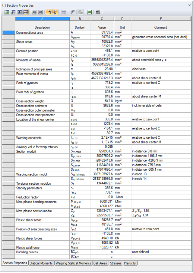
SHAPE-THIN determines the section properties and stresses of any open, closed, built-up, or non-connected cross-sections.
- Section Properties
- Cross-sectional area A
- Shear areas Ay, Az, Au, and Av
- Centroid position yS, zS
- moments of area 2 degrees Iy, Iz, Iyz, Iu, Iv, Ip, Ip,M
- Radii of gyration iy, iz, iyz, iu, iv, ip, ip,M
- Inclination of principal axes α
- Cross-section weight G
- Cross-section perimeter U
- torsional constants of area degrees IT, IT,St.Venant, IT,Bredt, IT,s
- Location of the shear center yM, zM
- Warping constants Iω,S, Iω,M or Iω,D for lateral restraint
- Max/min section moduli Sy, Sz, Su, Sv, Sω,M with locations
- Section ranges ru, rv, rM,u, rM,v
- Reduction factor λM
- Plastic Cross-Section Properties
- Axial force Npl,d
- Shear forces Vpl,y,d, Vpl,z,d, Vpl,u,d, Vpl,v,d
- Bending moments Mpl,y,d, Mpl,z,d, Mpl,u,d, Mpl,v,d
- Section moduli Zy, Zz, Zu, Zv
- Shear areas Apl,y, Apl,z, Apl,u, Apl,v
- Position of area bisecting axes fu, fv,
- Display of the inertia ellipse
- First moments of area Qu, Qv, Qy, Qz with location of maxima and specification of shear flow
- Warping coordinates ωM
- moments of area (warping areas) Sω,M
- Cell areas Am of closed cross-sections
- Normal stresses σx due to axial force, bending moments, and warping bimoment
- Shear stresses τ from shear forces as well as primary and secondary torsional moments
- Equivalent stresses σv with customizable factor for shear stresses
- Stress ratios, related to limit stresses
- Stresses for element edges or center lines
- Weld stresses in fillet welds
- Section properties of non-connected cross-sections (cores of high-rise buildings, composite sections)
- Shear wall shear forces due to bending and torsion
- Plastic capacity design with determination of the enlargement factor αpl
- Check of the c/t-ratios following the design methods el-el, el-pl or pl-pl according to DIN 18800
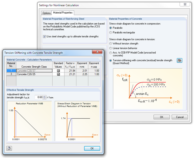
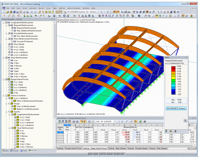
RF-CONCRETE Surfaces
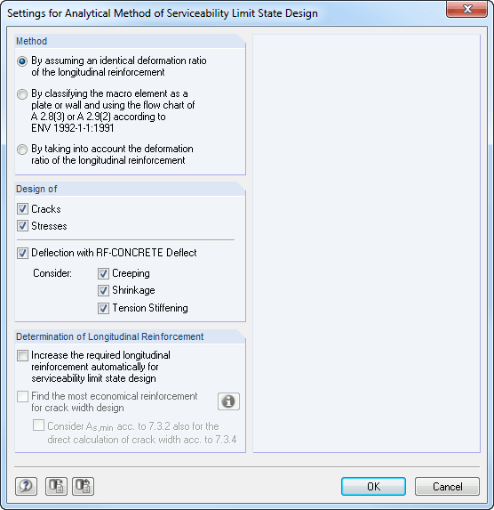
The nonlinear calculation is activated by selecting the design method of the serviceability limit state. You can individually select the analyses to be performed as well as the stress-strain diagrams for concrete and reinforcing steel. The iteration process can be influenced by these control parameters: convergence accuracy, maximum number of iterations, arrangement of layers over cross-section depth, and damping factor.
You can set the limit values in the serviceability limit state individually for each surface or surface group. Allowable limit values are defined by the maximum deformation, the maximum stresses, or the maximum crack widths. The definition of the maximum deformation requires additional specification as to whether the non-deformed or the deformed system should be used for the design.
RF-CONCRETE Members
The nonlinear calculation can be applied to the ultimate and the serviceability limit state designs. In addition, you can specify the concrete tensile strength or the tension stiffening between the cracks. The iteration process can be influenced by these control parameters: convergence accuracy, maximum number of iterations, and damping factor.
The deformation analysis according to the approximation method defined in standards (for example, deformation analysis according to EN 1992‑1‑1, 7.4.3) applies to the calculation of "effective stiffnesses" in the finite elements in accordance with the existing limit state of the concrete with or without cracks. These stiffnesses are used to determine the surface deformation by repeated FEM calculation.
The effective stiffness calculation of finite elements takes into account a reinforced concrete cross-section. Based on the internal forces determined for the serviceability limit state in RFEM, the program classifies the reinforced concrete cross-section as 'cracked' or 'uncracked'. If the tension stiffening at a section should be considered as well, a distribution coefficient (according to EN 1992-1-1, Eq. 7.19, for example) is used. The material behavior for the concrete is assumed to be linear-elastic in the compression and tension zone until the concrete tensile strength is reached. This is reached exactly in the serviceability limit state.
When determining the effective stiffnesses, creep and shrinkage are taken into account at the "cross-section level". The influence of shrinkage and creep in statically indeterminate systems is not taken into account in this approximation method (for example, tensile forces from shrinkage strain in systems restrained on all sides are not determined and must be considered separately). In summary, RF-CONCRETE Deflect calculates deformations in two steps:
- Calculation of effective stiffnesses of the reinforced concrete cross-section assuming linear-elastic conditions
- Calculation of the deformation using the effective stiffnesses with FEM
- Import of results from RSTAB
- Integrated material and cross-section library
- The module extension EC2 for RSTAB enables design of reinforced concrete according to EN 1992-1-1 (Eurocode 2) and the following National Annexes:
-
DIN EN 1992-1-1/NA/A1:2015-12 (Germany)
-
ÖNORM B 1992-1-1:2018-01 (Austria)
-
Belgium NBN EN 1992-1-1 ANB:2010 for design at normal temperature, and NBN EN 1992-1-2 ANB:2010 for fire resistance design (Belgium)
-
BDS EN 1992-1-1:2005/NA:2011 (Bulgaria)
-
EN 1992-1-1 DK NA:2013 (Denmark)
-
NF EN 1992-1-1/NA:2016-03 (France)
-
SFS EN 1992-1-1/NA:2007-10 (Finland)
-
UNI EN 1992-1-1/NA:2007-07 (Italy)
-
LVS EN 1992-1-1:2005/NA:2014 (Latvia)
-
LST EN 1992-1-1:2005/NA:2011 (Lithuania)
-
MS EN 1992-1-1:2010 (Malaysia)
-
NEN-EN 1992-1-1+C2:2011/NB:2016 (Netherlands)
- NS EN 1992-1 -1:2004-NA:2008 (Norway)
-
PN EN 1992-1-1/NA:2010 (Poland)
-
NP EN 1992-1-1/NA:2010-02 (Portugal)
-
SR EN 1992-1-1:2004/NA:2008 (Romania)
-
SS EN 1992-1-1/NA:2008 (Sweden)
-
SS EN 1992-1-1/NA:2008-06 (Singapore)
-
STN EN 1992-1-1/NA:2008-06 (Slovakia)
-
SIST EN 1992-1-1:2005/A101:2006 (Slovenia)
-
UNE EN 1992-1-1/NA:2013 (Spain)
-
CSN EN 1992-1-1/NA:2016-05 (Czech Republic)
-
BS EN 1992-1-1:2004/NA:2005 (United Kingdom)
-
CPM 1992-1-1:2009 (Belarus)
-
CYS EN 1992-1-1:2004/NA:2009 (Cyprus)
-
- In addition to the National Annexes (NA) listed above, you can also define a specific NA, applying user‑defined limit values and parameters.
- Optional presetting of partial safety factors, reduction factors, neutral axis depth limitation, material properties, and concrete cover
- Determination of longitudinal, shear, and torsional reinforcement
- Design of tapered members
- Cross‑section optimization
- Representation of minimum and compression reinforcement
- Determination of editable reinforcement proposal
- Crack width analysis with optional increase of the required reinforcement in order to keep the defined limit values of the crack width analysis
- Nonlinear calculation with consideration of cracked cross‑sections (for EN 1992‑1‑1:2004 and DIN 1045‑1:2008)
- Considering tension stiffening
- Considering creep and shrinkage
- Deformations in cracked sections (state II)
- Graphical representation of all result diagrams
- Fire resistance design according to the simplified method (zone method) according to EN 1992‑1‑2 for rectangular and circular cross‑sections. Thus, fire resistance design of brackets is possible as well.
The calculation can be performed for all member types according to the linear static, second-order, or large deformation analysis. This selection option is available for load cases and load combinations. Additional calculation parameters are individually adjustable for load cases, load combinations, and result combinations. This ensures a high degree of flexibility with regard to the calculation method and detailed specifications.
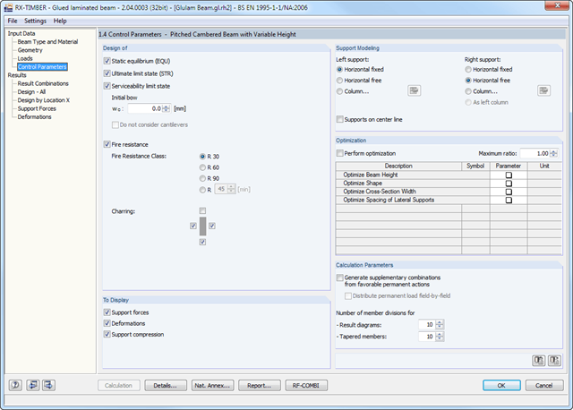
In RX-TIMBER Glued-Laminated Beam, the following calculation settings are available:
- Design of ULS, SLS, and/or fire resistance
- Selection of designs to be performed
- Determination of displaying support forces and deformations
- Adjusting the recommended limit values for the deformation analyses
- Definition of parameters for the fire resistance design performed according to the simplified method (optionally for F 30‑B, F 60‑B, F 90‑B, and user‑defined)
- Determination of tilting moment for pinned support
- Definition of support conditions for a beam
- Beam optimization by means of:
- Beam depth modification
- Modification of beam scene
- cross-section width
- Spacing of lateral supports