
The Ponding load type allows you to simulate rain actions on multi-curved surfaces, taking into account the displacements according to the large deformation analysis.
This numerical rainfall process examines the assigned surface geometry and determines which rainfall portions drain away and which rainfall portions accumulate in puddles (water pockets) on the surface. The puddle size then results in a corresponding vertical load for the structural analysis.
For example, you can use this feature in the analysis of approximately horizontal membrane roof geometries subjected to rain loading.
Go to Explanatory Video
Compared to the RF-FORM-FINDING add-on module (RFEM 5), the following new features have been added to the Form-Finding add-on for RFEM 6:
- Specification of all form-finding load boundary conditions in one load case
- Storage of form-finding results as initial state for further model analysis
- Automatic assignment of the form-finding initial state via combination wizards to all load situations of a design situation
- Additional form-finding geometry boundary conditions for members (unstressed length, maximum vertical sag, low-point vertical sag)
- Additional form-finding load boundary conditions for members (maximum force in member, minimum force in member, horizontal tension component, tension at i-end, tension at j-end, minimum tension at i-end, minimum tension at j-end)
- Material types "Fabric" and "Foil" in material library
- Parallel form-findings in one model
- Simulation of sequentially building form-finding states in connection with the Construction Stages Analysis (CSA) add-on

Once you activate the Form-Finding add-on in the Base Data, a form-finding effect is assigned to the load cases with the load case category "Prestress" in conjunction with the form-finding loads from the member, surface, and solid load catalog. This is a prestress load case. It thus mutates into a form-finding analysis for the entire model with all member, surface, and solid elements defined in it. You reach the form-finding of the relevant member and membrane elements amid the overall model by using special form-finding loads and regular load definitions. These form-finding loads describe the expected state of deformation or force after the form-finding in the elements. The regular loads describe the external loading of the entire system.
Do you know exactly how the form-finding is performed? First, the form-finding process of the load cases with the load case category "Prestress" shifts the initial mesh geometry to an optimally balanced position by means of iterative calculation loops. For this task, the program uses the Updated Reference Strategy (URS) method by Prof. Bletzinger and Prof. Ramm. This technology is characterized by equilibrium shapes that, after the calculation, comply almost exactly with the initially specified form-finding boundary conditions (sag, force, and prestress).
In addition to the pure description of the expected forces or sags on the elements to be formed, the integral approach of the URS also enables a consideration of regular forces. In the overall process, this allows, for example, for a description of the self-weight or a pneumatic pressure by means of corresponding element loads.
All these options give the calculation kernel the potential to calculate anticlastic and synclastic forms that are in an equilibrium of forces for planar or rotationally symmetric geometries. In order to be able to realistically implement both types individually or together in one environment, the calculation provide you with two ways to describe the form-finding force vectors:
- Tension method - description of the form-finding force vectors in space for planar geometries
- Projection method - description of the form-finding force vectors on a projection plane with fixation of the horizontal position for conical geometries

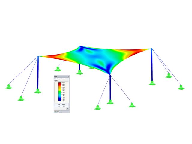
The form-finding process gives you a structural model with active forces in the "prestress load case" This load case shows the displacement from the initial input position to the form-found geometry in the deformation results. In the force or stress-based results (member and surface internal forces, solid stresses, gas pressures, and so on), it clarifies the state for maintaining the found form. For the analysis of the shape geometry, the program offers you a two-dimensional contour line plot with the output of the absolute height and an inclination plot for the visualization of the slope situation.
Now, a further calculation and structural analysis of the entire model is performed. For this purpose, the program transfers the form-found geometry including the element-wise strains into a universally applicable initial state. You can now use it in the load cases and load combinations.
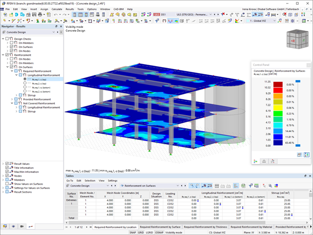
- Free definition of two reinforcement layers
- Design alternatives to avoid compression or shear reinforcement
- Design of surfaces as deep beams (theory of membranes)
- Option to define basic reinforcements for top and bottom reinforcement layers
- Free definition of provided surface reinforcement
- Result output in points of any selected grid
- Design with design moments at column edges
- Determination of deformation in state II; for example, according to EN 1992‑1‑1, 7.4.3, and ACI 318‑19 24.2.3, Table 24.2.3.5
- Considering tension stiffening
- Considering creep and shrinkage
- Fatigue design according to EN 1992‑1‑1, Chapter 6.8 (see this Product Feature)
- Design of a shear joint between the web and flange of ribs
- Optional pure slab or wall design of surfaces for a 2D model type
- Precise breakdown of reasons for failed design
- Design details of all design locations for better traceability of reinforcement determination

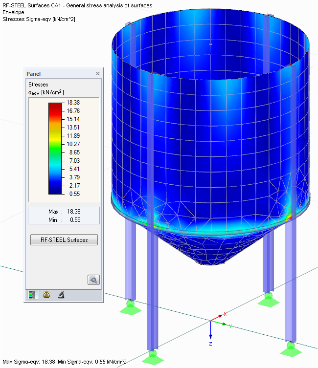
- Determination of principal and basic stresses, membrane and shear stresses, as well as equivalent stresses and equivalent membrane stresses
- Stress analysis for structural surfaces including simple or complex shapes
- Equivalent stresses calculated according to different approaches:
- Shape modification hypothesis (von Mises)
- Shear stress hypothesis (Tresca)
- Normal stress hypothesis (Rankine)
- Principal strain hypothesis (Bach)
- Optional optimization of surface thicknesses and data transfer to RFEM
- Output of strains
- Detailed results of individual stress components and ratios in tables and graphics
- Filter function for solids, surfaces, lines, and nodes in tables
- Transversal shear stresses according to Mindlin, Kirchhoff, or user-defined specifications
- Stress evaluation for welds at connection lines between surfaces (see the Product Feature)
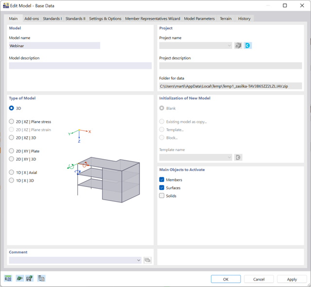
There are many options available for simple input and modeling. Your model is entered as a 1D, 2D, or 3D model. Member types such as beams, trusses, or tension members make it easier for you to define member properties. In order to model surfaces, RFEM provides you with various types, such as Standard, Without Thickness, Rigid, Membrane, and Load Distribution.
Furthermore, RFEM covers various material models, such as Isotropic | Linear Elastic, Orthotropic | Linear Elastic (Surfaces, Solids), or Isotropic | Timber | Linear Elastic (Members).
.png?mw=640&hash=9aa98962d5e0d0ed2803b35fcb6a2f87288b0946)
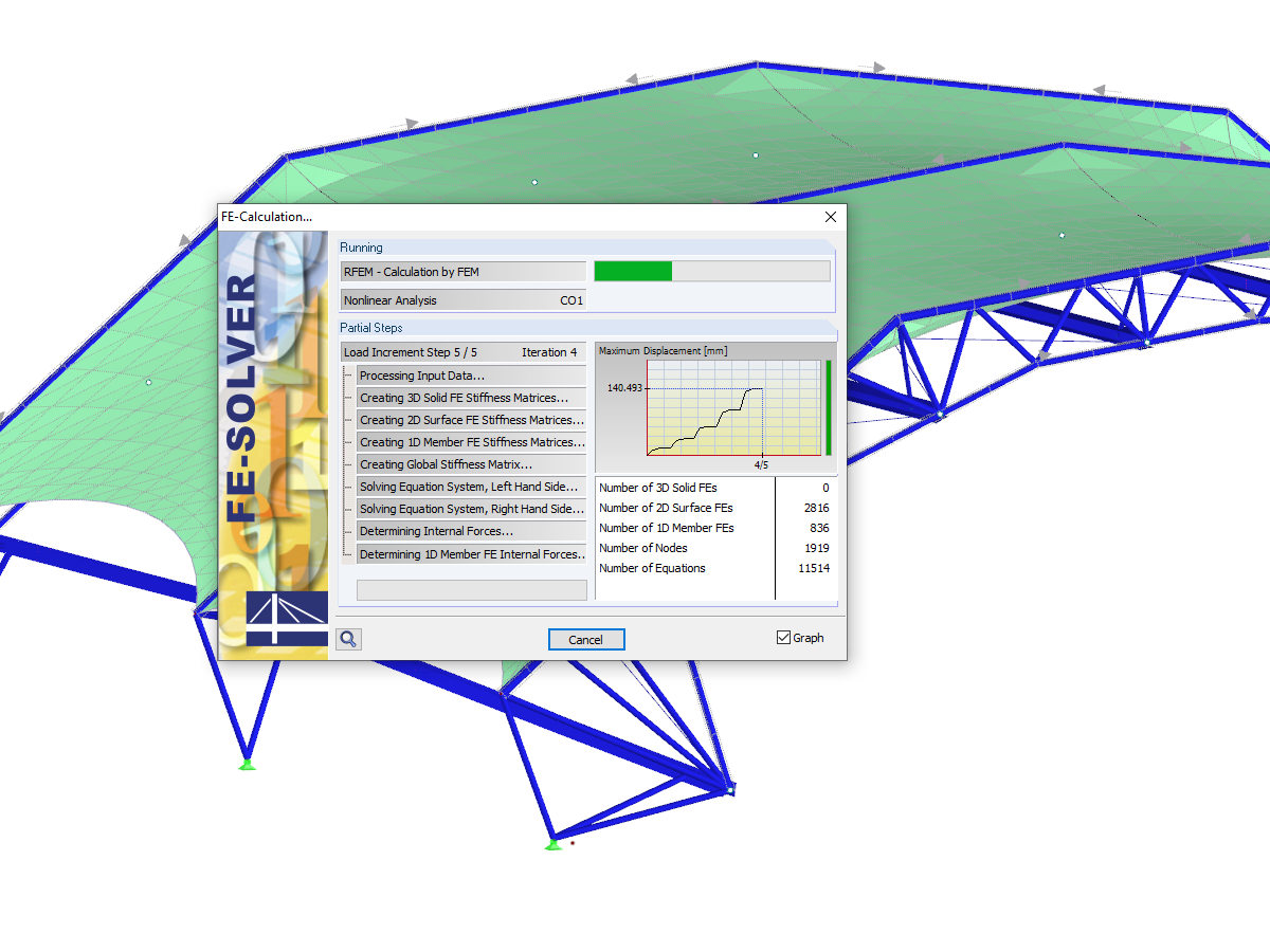
The number of degrees of freedom in a node is no longer a global calculation parameter in RFEM (6 degrees of freedom for each mesh node in 3D models, 7 degrees of freedom for the warping torsion analysis). Thus, each node is generally considered with a different number of degrees of freedom, which leads to a variable number of equations in the calculation.
This modification speeds up the calculation, especially for models where a significant reduction of the system could be achieved (for example, trusses and membrane structures).
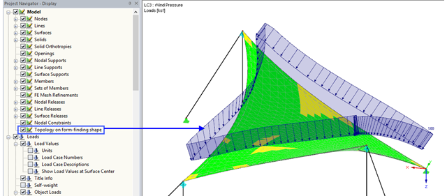
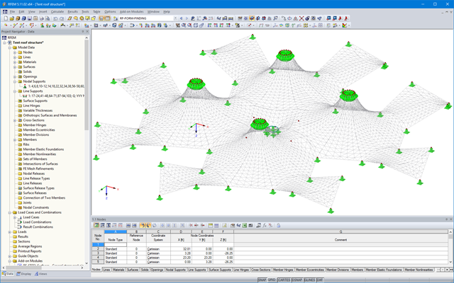
With the activated option 'Topology on Form-Finding Form' in Project Navigator - Display, the model display is optimized based on the form-finding geometry. For example, the loads are displayed in relation to the deformed system.
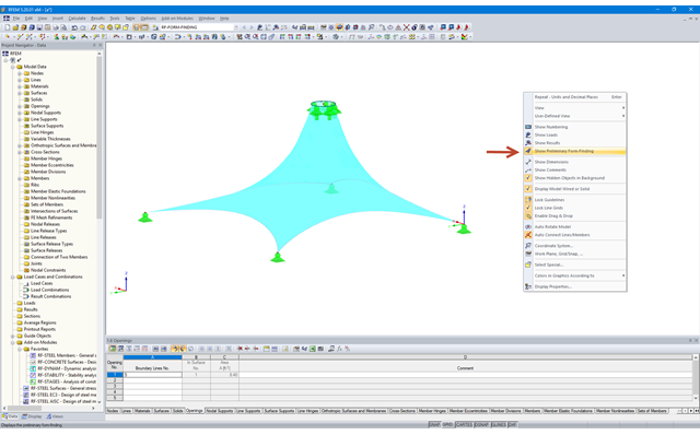
Activating 'Show Form-Finding' in the shortcut menu leads to an automatic preliminary form-finding according to the saved form-finding properties when you change the structure of membrane surfaces. This interactive graphics mode is based on the force density method.
More Information FAQ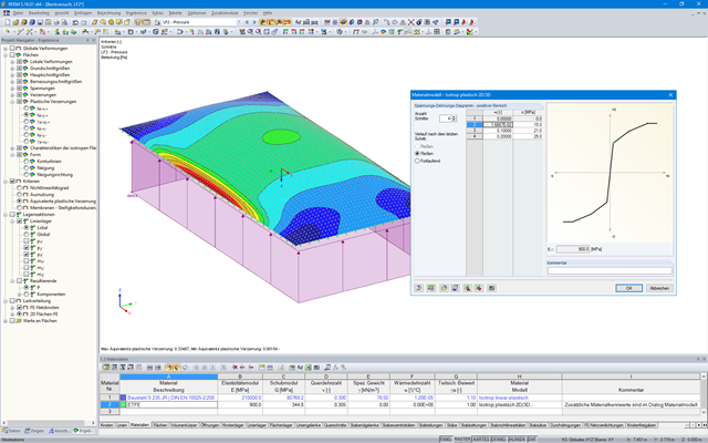
In RFEM, there is an option to couple surfaces with the stiffness types "Membrane" and "Membrane Orthotropic" with the material models "Isotropic Nonlinear Elastic 2D/3D" and "Isotropic Plastic 2D/3D" (add-on module RF-MAT NL is required).
This functionality enables simulation of the nonlinear strain behavior of ETFE foils, for example.
- Determination of principal and basic stresses, membrane and shear stresses, as well as equivalent stresses and equivalent membrane stresses
- Stress analysis for structural surfaces including simple or complex shapes
- Equivalent stresses calculated according to different approaches:
- Shape modification hypothesis (von Mises)
- Shear stress hypothesis (Tresca)
- Normal stress hypothesis (Rankine)
- Principal strain hypothesis (Bach)
- Optional optimization of surface thicknesses and data transfer to RFEM
- Serviceability limit state design by checking surface displacements
- Detailed results of individual stress components and ratios in tables and graphics
- Filter function for surfaces, lines, and nodes in tables
- Transversal shear stresses according to Mindlin, Kirchhoff, or user-defined specifications
- Parts list of designed surfaces
.png?mw=640&hash=688fdfc8af4828c08e9851cddb103a1e86cb899a)
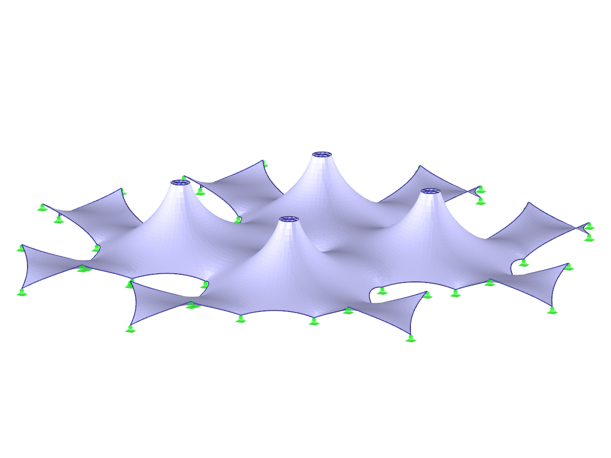
- Form-finding of:
- tension-loaded membrane and cable structures
- compression-loaded shell and beam structures
- mixed tension- and compression-loaded structures
- Consideration of gas chambers between surfaces
- Interaction with supporting structure (substructure design according to various standards)
- Surfaces as a 2D and members as a 1D element
- Definition of different prestress conditions for surfaces (membranes and shells)
- Definition of forces or geometrical requirements for members (cables and beams)
- Consideration of individual loads (self‑weight, inner pressure, and so on) in the form‑finding process
- Temporary support definitions for the form-finding process
- Automatic preliminary form-finding of membrane surfaces (more information...)
- Definition of isotropic or orthotropic material for structural analysis
- Optional definition of free polygon loads
- Transformation of form‑found shape elements into NURBS surface elements
- Possibility of combined form-finding by integration of preliminary form-finding
- Graphical evaluation of the new form using colored coordinates and inclination plots
- Complete documentation of the calculation including user-defined adaptive evaluation figures
- Optional export of the FE mesh as a DXF or Excel file

The nonlinear calculation adopts the real mesh geometry of planar, buckled, simple curved, or double curved surface components from the selected cutting pattern and flattens this surface component in compliance with the minimization of distortion energy, assuming defined material behavior.
In simplified terms, this method attempts to compress the mesh geometry in a press, assuming frictionless contact, and to find the state in which the stresses from flattening in the component are in equilibrium in the plane. This way, minimum energy and optimum accuracy of the cutting pattern are achieved. Compensation for warp and weft as well as compensation for boundary lines are considered. Then, the defined allowances on boundary lines are applied to the resulting planar surface geometry.
Features:
- Minimization of distortion energy in the flattening process for very accurate cutting patterns
- Application for almost all mesh arrangements
- Recognition of adjacent cutting pattern definitions to keep the same length
- Mesh application for main calculation
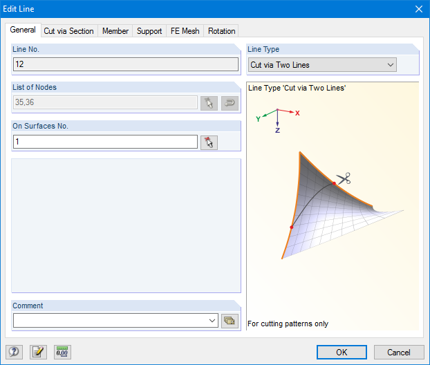
RF-CUTTING-PATTERN is activated by selecting the respective option in the Options tab in General Data of any RFEM model. After activating the add‑on module, a new object, "Cutting Patterns", is displayed under Model Data. If the membrane surface distribution for cutting in the basic position is too large, you can divide the surface by cutting lines (line types "Cut via Two Lines" or "Cut via Section") in the corresponding partial strips.
Then you can define the individual entries for each cutting pattern using the "Cutting Pattern" object. Here you can set boundary lines, compensations, and allowances.
Steps of the working sequence:
- Creation of cutting lines
- Creation of the pattern by selecting its boundary lines or using a semi‑automatic generator
- Free selection of warp and weft orientation by entering an angle
- Application of compensation values
- Optional definition of different compensations for boundary lines
- Different allowances (welding, boundary line)
- Preliminary representation of the cutting pattern in the graphic window at the side without starting the main nonlinear calculation
The results of the form‑finding process are a new shape and corresponding inner forces. The usual results, such as deformations, forces, stresses, and others can be displayed in the RF‑FORM‑FINDING case.
This prestressed shape is available as the initial state for all other load cases and combinations in the structural analysis.
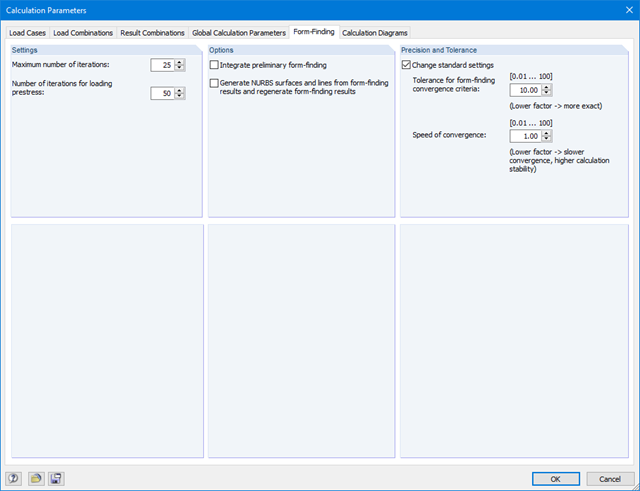
For more ease when defining load cases, the NURBS transformation can be used (Calculation Parameters/Form-Finding). This feature moves the original surfaces and cables into position after form‑finding.
By using the grid points of surfaces or the definition nodes of NURBS surfaces, free loads can be situated on selected parts of the structure.
The form-finding function can be activated in the General Data dialog box, Options tab. Prestresses (or geometrical requirements for members) can be defined in the parameters for surfaces and members. The form‑finding process is performed by calculation of an RF‑FORM‑FINDING case.
Steps of the working sequence:
- Creation of a model in RFEM (surfaces, beams, cables, supports, material definition, and so on)
- Setting of required prestress for membranes and force or length/sag for members (for example, cable)
- Optional consideration of other loads for the form-finding process in special form‑finding load cases (self‑weight, pressure, steel node weight, and so on)
- Setting of loads and load combinations for further structural analyses
- Planar and geodesic cutting lines
- Flattening of double-curved surface parts of tensioned membranes or pneumatic cushions
- Definition of cutting patterns by using boundary lines which are not required to be connected
- Sophisticated flattening based on the minimum energy theory
- Welding and boundary allowances
- Uniform or linear compensation in warp and weft direction
- Possibility of different compensations for boundary lines
- Adaptable data organisation (any additional modification of input data is considered up to the final "weld")
- Graphical display of cutting patterns
- Statistical information about each cutting pattern (width, length, size)
- Option to automatically generate cutting patterns from cells
After starting the calculation, the program performs form‑finding on the entire structure. The calculation takes into account the interaction between the form‑finding elements (membranes, cables, and so on) and the supporting structure.
The form-finding process is performed iteratively as a special nonlinear analysis, inspired by URS (Updated Reference Strategy) by Prof. Bletzinger / Prof. Ramm. This way, shapes in equilibrium are obtained considering the pre‑defined prestress.
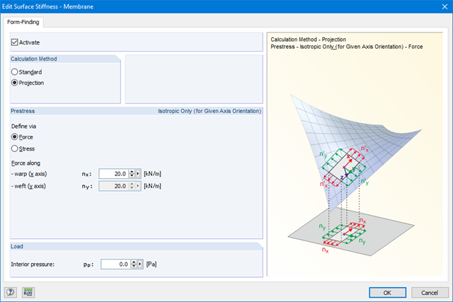
Furthermore, this method allows you to consider individual loads such as self‑weight or internal pressure for pneumatic structures in the form‑finding process. The prestress for surfaces (for example, membranes) can be defined using two different methods:
- Standard method - prescription of required prestress in a surface
- Projection method - prescription of required prestress in the projection of a surface, stabilization especially for conical shapes
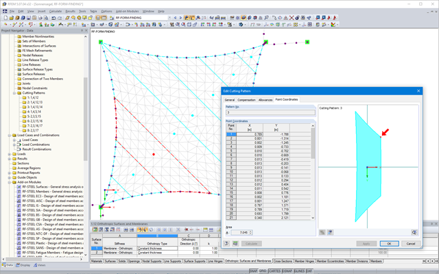
After the calculation, the "Point Coordinates" tab appears in the cutting pattern dialog box. In this tab, the result is displayed in the form of a table with coordinates and a surface in the graphical window. The coordinate table presents new flattened coordinates relative to the centroid of the cutting pattern for each mesh node. Furthermore, the cutting pattern with the coordinate system at the centroid is represented in the graphical window. When selecting a table cell, the respective node is displayed with an arrow in the graphic. In addition, the area of the cutting pattern is displayed below the node table.
Moreover, standard stress/strain results for each pattern are displayed in the RF‑CUTTING‑PATTERN load case in RFEM.
Features:
- Results in a table, including information about the cutting pattern
- Smart table relating to the graphic
- Results of flattened geometry in a DXF file
- Output of strains after flattening in order to evaluate the cutting patterns
- Results of strains after flattening for the evaluation of patterns
- Free definition of two or three reinforcement layers in the ultimate limit state
- Vectorial representation of the main stress directions of internal forces allowing optimal orientation adjustment of the third reinforcement layer to the actions
- Design alternatives to avoid compression or shear reinforcement
- Design of surfaces as deep beams (theory of membranes)
- Option to define basic reinforcements for top and bottom reinforcement layers
- Definition of designed reinforcement for serviceability limit state design
- Result output in points of any selected grid
- Optional extension of the module with nonlinear deformation analysis. The calculation is performed in RF‑CONCRETE Deflect by reducing the stiffness according to the standard, or in RF‑CONCRETE NL by the general nonlinear calculation determining the stiffness reduction in an iterative process.
- Design with design moments at column edges
- Precise breakdown of reasons for failed design
- Design details of all design locations for better traceability of reinforcement determination
- Export of isolines for the longitudinal reinforcement in a DXF file for further use in CAD programs as a basis for reinforcement drawings
The designs are carried out step-by-step by the eigenvalue calculation of the ideal buckling values for the individual stress states, as well as the buckling value for the simultaneous effect of all stress components.
The buckling analysis is based on the method of reduced stresses, comparing the acting stresses to a limit stress condition reduced from the yield condition of von Mises for each buckling panel. The design is based on a single global slenderness ratio determined by the entire stress field. Therefore, the design of single loading and subsequent merging using interaction criterion is omitted.
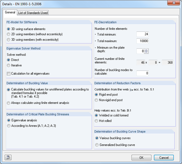
In order to determine the plate buckling behavior, which is similar to the behavior of a buckling member, the module calculates the eigenvalues of the ideal panel buckling values using freely assumed longitudinal edges. Then, slenderness ratios and reduction factors according to EN 1993-1-5, Ch. 4 or Annex B or DIN 18800, Part 3, Table 1. The design is then performed according to EN 1993-1-5, Chapter. 10 or DIN 18800, Part 3, Eq. (9), (10) or (14).
The buckling panel is discretized in finite quadrilateral or, if necessary, triangular elements. Each element node has six degrees of freedom.
The bending component of a triangular element is based on the LYNN-DHILLON element (2nd Conf. Matrix Meth. JAPAN – USA, Tokyo) according to the bending theory of Mindlin. However, the membrane component is based on the BERGAN-FELIPPA element. The quadrilateral elements consist of four triangular elements, while the inner node is eliminated.
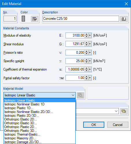
Structures are entered as 1D, 2D, or 3D models. Member types such as beams, trusses, or tension members facilitate the definition of member properties. For modeling surfaces, RFEM provides For example, the types Standard, Orthotropic, Glass, Laminate, Rigid, Membrane, and so on, are available.
Furthermore, RFEM can select among the material models Isotropic Linear Elastic, Isotropic Plastic 1D/2D/3D, Isotropic Nonlinear Elastic 1D/2D/3D, Orthotropic Elastic 2D/3D, Orthotropic Plastic 2D/3D (Tsai-Wu 2D/3D), and Isotropic Thermal -elastic, Isotropic Masonry 2D, and Isotropic Damage 2D/3D.