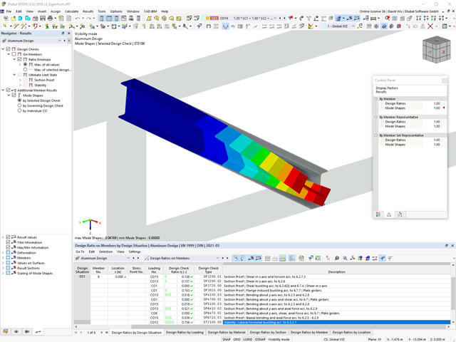
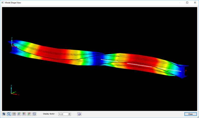
Did you use the eigenvalue solver of the add-on to determine the critical load factor within the stability analysis? In this case, you can then display the governing mode shape of the object to be designed as a result.
- Stability analyses for flexural buckling, torsional buckling, and flexural-torsional buckling under compression
- Import of the effective lengths from the calculation using the Structure Stability add-on
- Graphical input and check of the defined nodal supports and effective lengths for stability analysis
- Determination of the equivalent member lengths for tapered members
- Consideration of Lateral-Torsional Bracing Position
- Lateral-torsional buckling analysis of the structural components subjected to moment loading
- Depending on the standard, a choice between user-defined input of Mcr, analytical method from the standard, and use of internal eigenvalue solver
- Consideration of a shear panel and a rotational restraint when using the eigenvalue solver
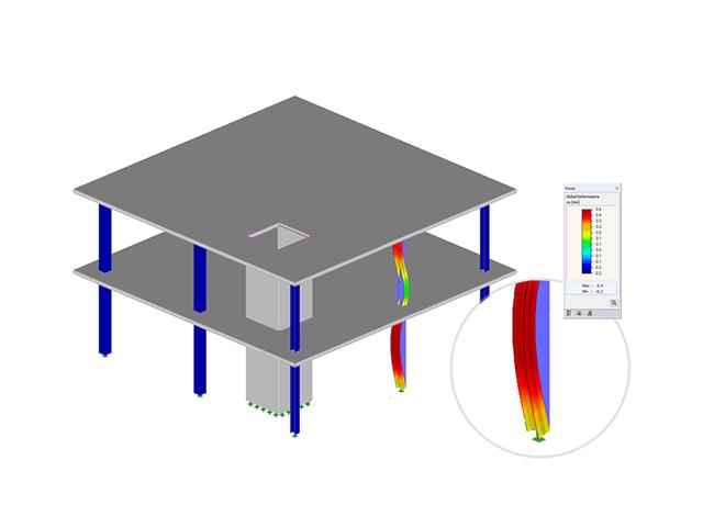
- Graphical display of a mode shape if the eigenvalue solver was used
- Stability analysis of structural components with the combined compression and bending stress, depending on the design standard
- Comprehensible calculation of all necessary coefficients, such as the factors for considering moment distribution or interaction factors
- Alternative consideration of all effects for the stability analysis when determining internal forces in RFEM/RSTAB (second-order analysis, imperfections, stiffness reduction, possibly in combination with the Torsional Warping (7 DOF) add-on)
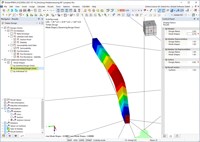
Did you use the eigenvalue solver of the add-on to determine the critical load factor within the stability analysis? If so, you can then display the governing mode shape of the object to be designed as a result. The eigenvalue solver is available here for the lateral-torsional buckling analysis, depending on the design standard used.
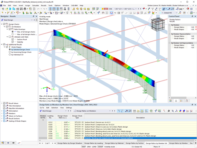
Did you use the eigenvalue solver of the add-on to determine the critical load factor for the stability analysis? Verz well, you can then display the governing mode shape of the object to be designed as a result. The eigenvalue solver is available for the lateral-torsional buckling analysis, depending on the design standard used. You can also use the internal eigenvalue solver for the general method according to EN 1993‑1‑1, 6.3.4.

- Calculation of stationary incompressible turbulent wind flow using the SimpleFOAM solver from the OpenFOAM® software package
- Numerical scheme according to the first and second order
- Turbulence models RAS k-ω and RAS k-ε
- Consideration of surface roughness depending on model zones
- Model design via VTP, STL, OBJ, and IFC files
- Operation via bidirectional interface of RFEM or RSTAB for importing model geometries with standard-based wind loads and exporting wind load cases with probe-based printout report tables
- Intuitive model changes via drag & drop and graphical adjustment assistance
- Generation of a shrink-wrap mesh envelope around the model geometry
- Consideration of environmental objects (buildings, terrain, and so on)
- Height-dependent description of the wind load (wind speed and turbulence intensity)
- Automatic meshing depending on a selected depth of detail
- Consideration of layer meshes near the model surfaces
- Parallelized calculation with optimal utilization of all processor cores of a computer
- Graphical output of the surface results on the model surfaces (surface pressure, Cp coefficients)
- Graphical output of the flow field and vector results (pressure field, velocity field, turbulence – k-ω field, and turbulence – k-ε field, velocity vectors) on Clipper/Slicer planes
- Display of 3D wind flow via animated streamline graphics
- Definition of point and line probes
- Multilingual user interface (German, English, Czech, Spanish, French, Italian, Polish, Portuguese, Russian, and Chinese)
- Calculations of several models in one batch process
- Generator for creating rotated models to simulate different wind directions
- Optional interruption and continuation of the calculation
- Individual color panel per result graphic
- Display of diagrams with separate output of results on both sides of a surface
- Output of the dimensionless wall distance y+ in the mesh inspector details for the simplified model mesh
- Determination of the shear stress on the model surface from the flow around the model
- Calculation with an alternative convergence criterion (you can select between the residual types pressure or flow resistance in the simulation parameters)
- Calculation of transient incompressible turbulent wind flow with the BlueDyMSolver solver
- LES SpalartAllmarasDDES turbulence model
- Consideration of stationary solution as initial state for transient calculation
- Automatic determination of analysis period and time steps
- Use of intermediate results during the calculation
- Organized display of time-varying results via time step units
- Diagram of drag force and point probe results over analysis time
- Display of line probe results for any time steps in a diagram
- Freely adjustable wind permeability for surfaces (Go to Product Feature)
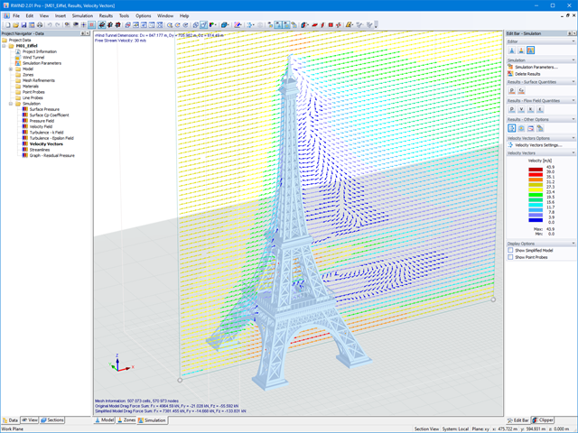
RWIND Basic uses a numerical CFD model (Computational Fluid Dynamics) to simulate wind flows around your objects using a digital wind tunnel. The simulation process determines specific wind loads acting on your model surfaces from the flow result around the model.
A 3D volume mesh is responsible for the simulation itself. For this, RWIND Basic performs an automatic meshing on the basis of freely definable control parameters. For the calculation of wind flows, RWIND Basic provides you with a stationary solve and RWIND Pro provides a transient solver for incompressible turbulent flows. Surface pressures resulting from the flow results are extrapolated onto the model for each time step.
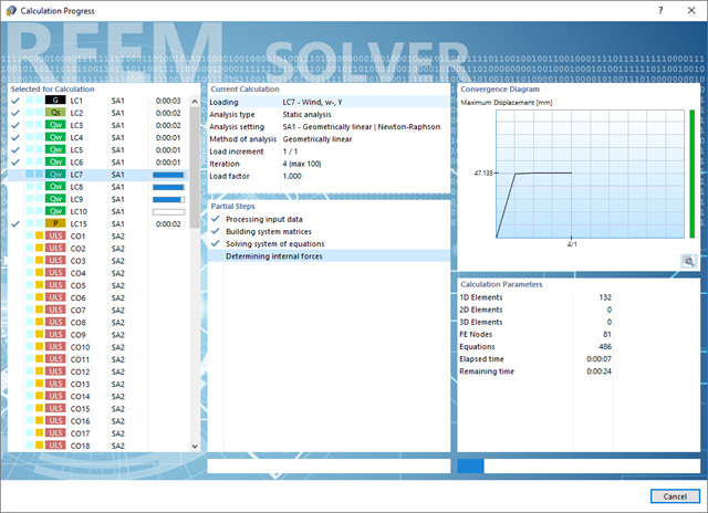
Do you have to calculate multiple load combinations in your models? Then several solvers (one per core) are initiated in parallel, each of which calculates a load combination. This ensures a better utilization of the cores and thus faster calculations.
Go to Explanatory Video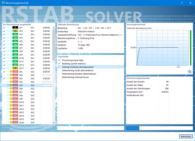
Also in this case, RSTAB will certainly convince you. With the powerful calculation kernel, its optimized networking and support of multi-core processor technology, the Dlubal structural analysis program is far ahead. This allows you to calculate more linear load cases and load combinations using several processors in parallel without using additional memory. The stiffness matrix only has to be created once. Thus, it is possible for you to calculate even large systems with the fast and direct solver.
Do you have to calculate multiple load combinations in your models? The program initiates several solvers in parallel (one per core). Each solver then calculates a load combination for you. This leads to better utilization of the cores.
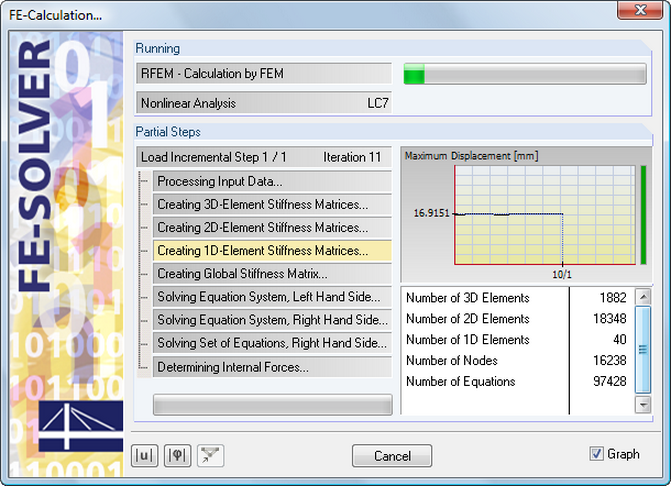
You can systematically follow the development of the deformation displayed in a diagram during the calculation, and thus precisely evaluate the convergence behavior.
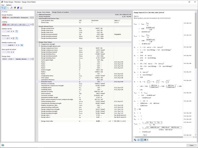
Compared to the RF‑/TIMBER Pro add-on module (RFEM 5 / RSTAB 8), the following new features have been added to the Timber Design add-on for RFEM 6 / RSTAB 9:
- In addition to Eurocode 5, other international standards are integrated (SIA 265, ANSI/AWC NDS, CSA O86, GB 50005)
- Design of compression perpendicular to grain (support pressure)
- Implementation of eigenvalue solver for determining the critical moment for lateral-torsional buckling (EC 5 only)
- Definition of different effective lengths for design at normal temperature and fire resistance design
- Evaluation of stresses via unit stresses (FEA)
- Optimized stability analyses for tapered members
- Unification of the materials for all national annexes (only one "EN" standard is now available in the material library for a better overview)
- Display of cross-section weakenings directly in the rendering
- Output of the used design check formulas (including a reference to the used equation from the standard)

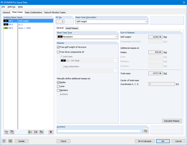
In the modal analysis settings, you have to enter all data that are necessary for the determination of the natural frequencies. These are, for example, mass shapes and eigenvalue solvers.
The Modal Analysis add-on determines the lowest eigenvalues of the structure. Either you adjust the number of eigenvalues or let them determined automatically. Thus, you should reach either effective modal mass factors or maximum natural frequencies. Masses are imported directly from load cases and load combinations. In this case, you have the option to consider the total mass, load components in the global Z-direction, or only the load component in the direction of gravity.
You can manually define additional masses at nodes, lines, members, or surfaces. Furthermore, you can influence the stiffness matrix by importing axial forces or stiffness modifications of a load case or load combination.

In RFEM, you can use these three powerful eigenvalue solvers:
- Root of Characteristic Polynomial
- Method by Lanczos
- Subspace Iteration
RSTAB, on the other hand, provides you with these two eigenvalue solvers:
- Subspace Iteration
- Shifted inverse power method
The selection of the eigenvalue solver depends primarily on your model size.
- Stability analyses for flexural buckling, torsional buckling, and flexural-torsional buckling under compression
- Import of the effective lengths from the calculation using the Structure Stability add-on
- Graphical input and check of the defined nodal supports and effective lengths for stability analysis
- Lateral-torsional buckling analysis of the structural components subjected to moment loading
- Depending on the standard, a choice between user-defined input of Mcr, analytical method from the standard, and use of internal eigenvalue solver
- Consideration of a shear panel and a rotational restraint when using the eigenvalue solver
- Graphical display of a mode shape if the eigenvalue solver was used
- Stability analysis of structural components with the combined compression and bending stress, depending on the design standard
- Comprehensible calculation of all necessary coefficients, such as the factors for considering moment distribution or interaction factors
- Alternative consideration of all effects for the stability analysis when determining internal forces in RFEM/RSTAB (second-order analysis, imperfections, stiffness reduction, possibly in combination with the Torsional Warping (7 DOF) add-on)

- Stability analyses for flexural buckling, torsional buckling, and flexural-torsional buckling under compression
- Lateral-torsional buckling analysis of the structural components subjected to moment loading
- Import of the effective lengths from the calculation using the Structure Stability add-on
- Graphical input and check of the defined nodal supports and effective lengths for stability analysis
- Depending on the standard, a choice between user-defined input of Mcr, analytical method from the standard, and use of internal eigenvalue solver
- Consideration of a shear panel and a rotational restraint when using the eigenvalue solver
- Graphical display of a mode shape if the eigenvalue solver was used
- Stability analysis of structural components with the combined compression and bending stress, depending on the design standard
- Comprehensible calculation of all necessary coefficients, such as interaction factors
- Alternative consideration of all effects for the stability analysis when determining internal forces in RFEM/RSTAB (second-order analysis, imperfections, stiffness reduction, possibly in combination with the Torsional Warping (7 DOF) add-on)

- Calculation of models consisting of member, shell, and solid elements
- Nonlinear stability analysis
- Optional consideration of axial forces from initial prestress
- Four equation solvers for an efficient calculation of various structural models
- Optional consideration of stiffness modifications in RFEM/RSTAB
- Determination of a stability mode greater than the user-defined load increment factor (Shift method)
- Optional determination of the mode shapes of unstable models (to identify the cause of instability)
- Visualization of the stability mode
- Basis for determining imperfection
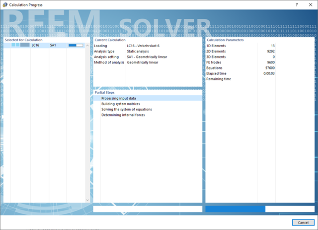
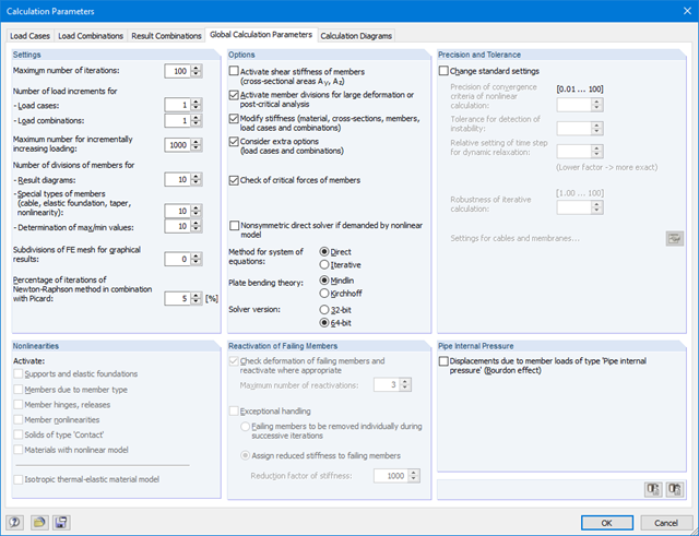
Convince yourself by the powerful calculation kernel, its optimized networking and support of multi-core processor technology. This provides you with the advantages, such as parallel calculations of linear load cases and load combinations using several processors without additional demands on the RAM. The stiffness matrix only has to be created once. Thus, you can calculate even large systems with the fast direct solver.
If you need to calculate multiple load combinations in your models, the program initiates several solvers in parallel (one per core). Each solver then calculates a load combination, which improves the core utilization.
You can systematically follow the development of the deformation displayed in a diagram during the calculation, and thus precisely evaluate the convergence behavior.
Work on your models with efficient and precise calculations in the digital wind tunnel. RWIND 2 uses a numerical CFD model (Computational Fluid Dynamics) to simulate wind flows around objects. Specific wind loads are generated from the simulation process for RFEM or RSTAB.
RWIND 2 performs this simulation using a 3D volume mesh. The program provides automatic meshing; you can easily set the entire mesh density as well as the local mesh refinement on the model using a few parameters. A numerical solver for incompressible turbulent flows is used to calculate the wind flows and the surface pressures on the model. The results are then extrapolated to your model. RWIND 2 is designed to work with different numerical solvers.
We currently recommend using the OpenFOAM® software package, which has provided very good results in our tests and is also a frequently used tool for CFD simulations. Alternative numerical solvers are under development.
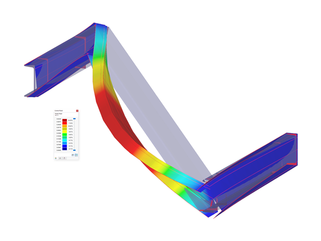
The determination of the critical buckling moment is carried out in RF-/STEEL AISC by using the eigenvalue solver which allows an exact determination of the critical buckling load.
The eigenvalue solver shows a display window of the eigenvalue graphics, which enables checking of the boundary conditions.
- Applicable for members defined as sets of members
- Separate solver that considers 7 deformation directions (ux, uy, uz, φx, φy, φz, ω) or 8 internal forces (N, Vu, Vv, Mt,pri, Mt,sec, Mu, Mv, Mω)
- Nonlinear design according to second-order analysis
- Input of imperfections
- Calculation of critical load factors and buckling mode shapes as well as the visualization of them (incl. warping)
- Integration into member design in the RF-/STEEL AISC and RF‑/STEEL EC3 add‑on modules
- Available for all thin‑walled steel cross‑sections
The equation solver includes an optimized FE mesh generator and supports the latest multi-core processor and 64-bit technology. It enables parallel calculations of linear load cases and load combinations using several processors without additional demands on the RAM: The stiffness matrix only has to be created once. The 64-bit technology and the enhanced RAM options allow for calculation of complex structural systems using the fast and direct equation solver.
The development of the deformation is displayed in a diagram during the calculation. This way, you can easily evaluate the convergence behavior.
Several methods are available for the eigenvalue analysis:
- Direct Methods
- The direct methods (Lanczos, roots of characteristic polynomial, subspace iteration method) are suitable for small to medium-sized models. These fast methods for equation solvers benefit from a lot of the computer memory (RAM). 64-bit systems use more memory so that even bigger structural systems can be calculated quickly.
- ICG iteration method (Incomplete Conjugate Gradient)
- This method requires only a small amount of memory. Eigenvalues are determined one after the other. It can be used to calculate large structural systems with few eigenvalues.
The RF-STABILITY add-on module can also perform the non-linear stability analysis. Also for nonlinear structures, results close to reality are provided. The critical load factor is determined by gradually increasing the loads of the underlying load case until the instability is reached. The load increment takes into account nonlinearities such as failing members, supports and foundations, and material nonlinearities.

You can select several methods that are available for the eigenvalue analysis:
- Direct Methods
- The direct methods (Lanczos [RFEM], roots of characteristic polynomial [RFEM], subspace iteration method [RFEM/RSTAB], and shifted inverse iteration [RSTAB]) are suitable for small to medium-sized models. You should only use these fast solver methods if your computer has a larger amount of memory (RAM).
- ICG Iteration Method (Incomplete Conjugate Gradient [RFEM])
- In contrast, this method only requires a small amount of memory. Eigenvalues are determined one after the other. It can be used to calculate large structural systems with few eigenvalues.
Use the Structure Stability add-on to perform a nonlinear stability analysis using the incremental method. This analysis delivers close-to-reality results also for nonlinear structures. The critical load factor is determined by gradually increasing the loads of the underlying load case until the instability is reached. The load increment takes into account nonlinearities such as failing members, supports and foundations, and material nonlinearities. After increasing the load, you can optionally perform a linear stability analysis on the last stable state in order to determine the stability mode.
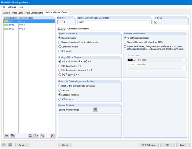
The RF-DYNAM Pro - Natural Vibrations module of RFEM provides four powerful eigenvalue solvers:*Root of characteristic polynomial
- Method by Lanczos
- Subspace Iteration
- ICG iteration method (Incomplete Conjugate Gradient)
The DYNAM Pro - Natural Vibrations module for RSTAB provides two eigenvalue solvers:
- Subspace Iteration
- Shifted inverse power method
The selection of the eigenvalue solver depends primarily on the size of the model.
Input windows require all data necessary for determination of natural frequencies, such as mass shapes and eigenvalue solvers.
The RF-/DYNAM Pro - Natural Vibrations add-on module determines the lowest eigenvalues of the structure. The number of eigenvalues can be adjusted. Masses are directly imported from load cases or load combinations (with optional consideration of total masses or a load component in the direction of gravity).
Additional masses can be defined manually at nodes, lines, members, or surfaces. Furthermore, it is possible to control the stiffness matrix by importing normal forces or stiffness modifications of a load case or combination.
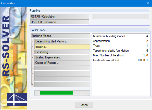
RSBUCK determines the most unfavorable buckling modes of a structure. It is generally not possible in terms of the calculation method to exclude lower eigenvalues from the analysis and at the same time, to attempt to determine higher eigenvalues. With RSBUCK, you can determine up to the 10,000 lowest eigenvalues of a structural system.
By default, RSBUCK uses the average value of the axial forces occurring on the individual members to calculate the eigenvalues/critical load factors. Optionally, the module can also process the most unfavorable axial force of a member. The determination of buckling modes is performed by an eigenvalue analysis for the entire structure. For this, an iterative equation solver is used.
You only have to specify the following two values:
- the maximum number of iterations
- the break-off limit
Since an exact solution is approximated as close as desired, but never reached, RSBUCK terminates the calculation process after the specified number of iteration steps. In the case of a convergence problem, the break-off limit determines the moment when an approximate solution can be considered as an exact result. Divergence problems have no solution.
- Calculation of models consisting of member, shell, and solid elements
- Import of axial forces from a load case or combination
- Non-linear stability analysis
- Optional consideration of axial forces from initial prestress
- Four equation solvers for effective calculation of various structural models
- Optional consideration of stiffness modifications in RFEM
- Calculation of buckling modes of unstable models
- Determination of stability mode greater than the user-defined load increment factor (Shift method)
- Optional determination of the mode shapes of unstable models (to identify the cause of instability)
- Visualization of stability mode
- Basis for analysis using imperfect equivalent structures in RF-IMP