106 Wyniki
Wyświetl wyniki:
Sortuj według:
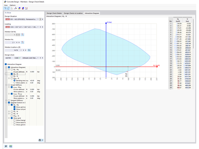
Czy wiesz, że wykresy interakcji moment-siła (wykresy MN) można wyświetlić również graficznie? Umożliwia to wyświetlenie nośności przekroju w przypadku interakcji momentu zginającego i siły osiowej. Oprócz wykresów interakcji związanych z osiami przekroju (wykres My-N i wykres Mz-N) można również wygenerować indywidualny wektor momentów w celu utworzenia wykresu interakcji Mres -N. Płaszczyznę przekroju wykresów MN można wyświetlić na wykresie interakcji 3D.Program wyświetla odpowiednie pary wartości stanu granicznego nośności w tabeli. Tabela jest dynamicznie powiązana z wykresem, dzięki czemu wybrany punkt graniczny jest również wyświetlany na wykresie.
Model budynku jest obliczany w dwóch etapach:
- Globale 3D-Berechnung des Gesamtmodells, in welchem die Decken als starre Ebene (Diaphragma) oder als Biegeplatte modelliert werden
- Lokale 2D-Berechnung der einzelnen Geschossdecken
Die Ergebnisse der Stützen und Wände aus der 3D-Berechnung und die Ergebnisse der Decken aus der 2D-Berechnung werden nach der Berechnung in einem einzigen Modell zusammengefasst. Dadurch muss zwischen dem 3D-Modell und der einzelnen 2D-Modellen der Decken nicht gewechselt werden. Der Anwender arbeitet nur mit einem Model, spart wertvolle Zeit und vermeidet eventuelle Fehler beim händischen Datenaustausch zwischen dem 3D-Modell und der einzelnen 2D-Decken-Modelle.
Die vertikalen Flächen im Modell können vom Nutzer in Schubwände (Shear Walls) und Öffnungsstürze (Sprandels) geteilt werden. Aus diesen Wandobjekten erzeugt das Programm automatisch interne Ergebnisstäbe, so dass diese dann nach der gewünschten Norm im Add-On Betonbemessung für RFEM 6 als Stäbe bemessen werden können.
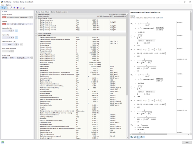
Dzięki oprogramowaniu Dlubal zawsze masz podgląd, niezależnie od tego, czy masz projekty z branży żelbetowej, stalowej, drewnianej, aluminiowej czy innej. Wzory do kontroli warunków projektowych zastosowane w obliczeniach są wyświetlane w przejrzysty sposób (wraz z odniesieniem do zastosowanego równania z normy). Te wzory do kontroli obliczeń można również uwzględnić w raporcie.
Przejdź do filmu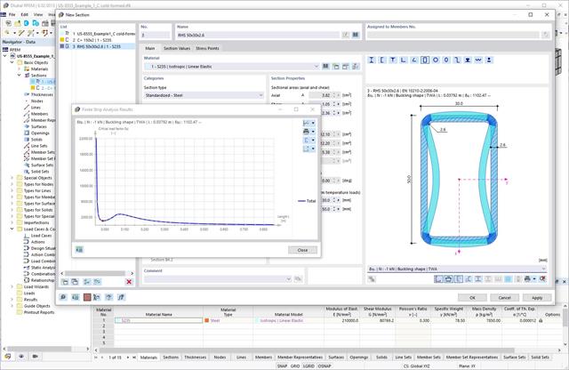
Podczas wymiarowania zgodnie z EN 1993-1-3, możliwe jest przedstawienie graficzne postaci własnej wyboczenia dystorsyjnego przekroju oraz dla przekrojów RSECTION.
Kształt postaci własnej można również wyprowadzić w RSECTION 1 dla przekrojów z biblioteki.
- 002469
- Ogólne informacje
- Projektowanie konstrukcji betonowych RFEM 6
- Projektowanie konstrukcji betonowych RSTAB 9
Pracujesz z elementami konstrukcyjnymi składającymi się z płyt? W takim przypadku należy przeprowadzić obliczenia na ścinanie z uwzględnieniem wymagań obliczania przebicia, na przykład zgodnie z 6.4, EN 1992-1-1. Oprócz płyt stropowych można w ten sposób wymiarować również płyty fundamentowe.
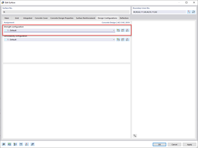
W konfiguracji stanu granicznego nośności dla wymiarowania betonu można zdefiniować parametry obliczeń przebicia dla wybranych węzłów.
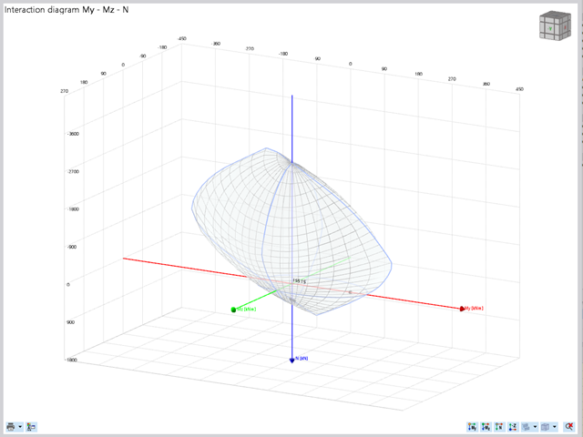
Projektowanie konstrukcji betonowych | Wykres interakcji My-Mz-N (3D) przekrojów z betonu zbrojonego
Na pytanie 'Ile można przewozić?' zazwyczaj odpowiada 'Tak'. Do graficznego przedstawiania stanu granicznego nośności przekrojów żelbetowych wymagany jest trójwymiarowy wykres interakcji momentu-momentu-siła osiowa. Oprogramowanie do analizy statyczno-wytrzymałościowej firmy Dlubal właśnie to oferuje.
Dzięki dodatkowemu wyświetleniu oddziaływania obciążenia można łatwo rozpoznać lub zwizualizować przekroczenie granicznej nośności przekroju żelbetowego. Ponieważ możesz kontrolować właściwości wykresu, możesz dostosować wygląd wykresu My-Mz-N do swoich potrzeb.
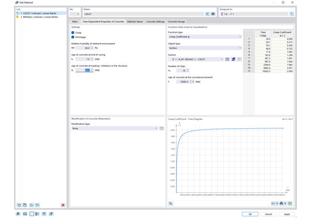
Właściwości betonu, zależne od czasu, takie jak pełzanie i skurcz, są bardzo ważne dla obliczeń. Można je zdefiniować bezpośrednio dla materiału w programie do analizy statyczno-wytrzymałościowej. W oknie dialogowym do wprowadzania danych wyświetlany jest przebieg czasowy funkcji pełzania lub skurczu. Można łatwo wybrać modyfikację zastosowanego wieku betonu, na przykład ze względu na obróbkę termiczną.
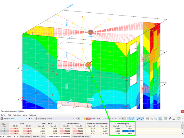
Aktywowałeś rozszerzenie Model budynku ? Bardzo dobrze! Możesz wyświetlić środek sztywności w tabeli i w formie graficznej. Użyj go na przykład do analizy dynamicznej.
- 002567
- Ogólne informacje
- Projektowanie konstrukcji stalowych RFEM 6
- Projektowanie konstrukcji stalowych RSTAB 9
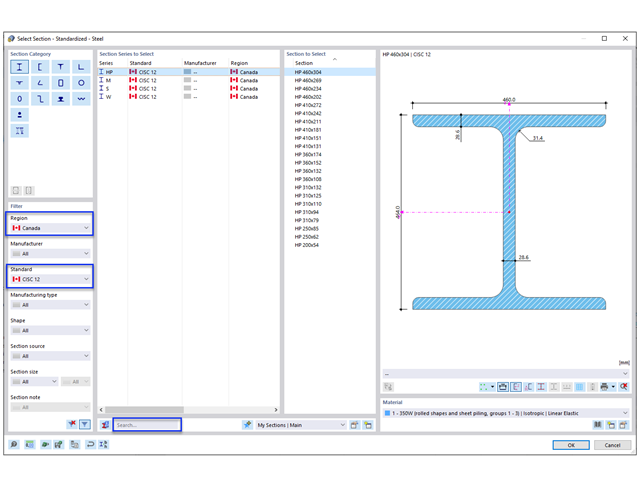
Nowe przekroje stalowe zgodnie z najnowszą instrukcją CISC (12 wydanie) są dostępne w programie RFEM 6. Przekroje są wymienione w bibliotece Znormalizowane. W filtrze należy wybrać region „Kanada”, a normę „CISC 12”. Alternatywnie nazwę przekroju można wprowadzić bezpośrednio w polu wyszukiwania znajdującym się w dolnej części okna dialogowego.
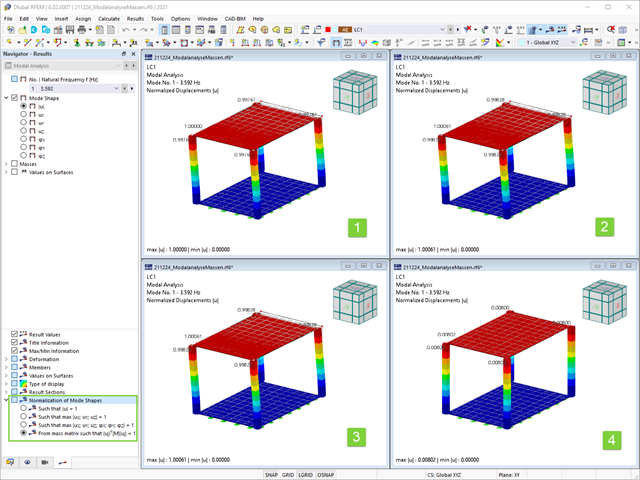
Jak już wiesz, po pomyślnym zakończeniu obliczeń wyniki przypadku obciążenia w Analizie modalnej są wyświetlane w programie. Die erste Eigenform ist für Sie also sofort grafisch oder animiert zu sehen. Dabei können Sie die Darstellung der Eigenformnormierung komfortabel anpassen. Erledigen Sie das am besten direkt im Ergebnisnavigator, wo Sie zur Visualisierung der Eigenformen eine von vier Optionen auswählen:
- Wert des Eigenformvektors uj auf 1 skalieren (berücksichtigt nur die Translationskomponenten)
- Auswahl der maximalen Translationskomponente des Eigenvektors und Einstellung auf 1
- Betrachtung der gesamten Eigenform (inklusive der Rotationskomponenten), Auswahl des Maximums und Einstellung auf 1
- Setzen der modalen Massen mi für jeden Eigenwert auf 1 kg
Ausführlichere Erläuterungen der Normierung der Eigenformen finden Sie hier: Instrukcja online .
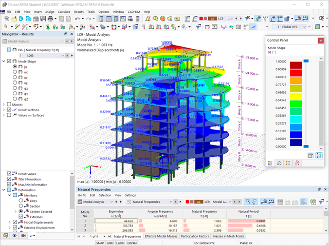
Czy obliczenia się zakończyły? Wyniki analizy modalnej są wówczas dostępne zarówno w formie graficznej, jak i tabelarycznej. Wyświetl tabele wyników dla przypadku obciążenia lub przypadków obciążeń analizy modalnej. Dzięki temu na pierwszy rzut oka można zobaczyć wartości własne, częstotliwości kątowe, częstotliwości i okresy drgań własnych konstrukcji. W przejrzysty sposób wyświetlane są również efektywne masy modalne, modalne współczynniki masy i współczynniki udziału.
.png?mw=640&hash=5a991f211d984ac624978f514e70c53da263e5d9)
W zależności od siły osiowej N, można wygenerować linię krzywizny momentu dla dowolnego wektora momentu. Program pokazuje również pary wartości wyświetlanego wykresu w tabeli. Ponadto można aktywować jako dodatkowy wykres sieczny i sztywność styczną przekroju żelbetowego, należące do wykresu krzywizny momentu.
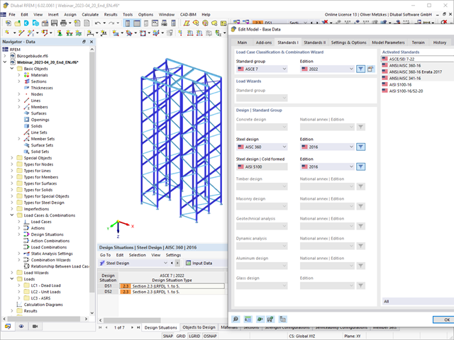
Wymiarowanie prętów stalowych formowanych na zimno zgodnie z AISI S100-16/CSA S136-16 jest dostępne w RFEM 6. Dostęp do obliczeń można uzyskać, wybierając normy „AISC 360” lub „CSA S16” w rozszerzeniu Projektowanie konstrukcji stalowych. Następnie dla obliczeń elementów formowanych na zimno automatycznie wybierane jest „AISI S100” lub „CSA S136”.
Do obliczania sprężystego obciążenia wyboczeniowego pręta program RFEM stosuje metodę DSM. Bezpośrednia metoda wytrzymałości oferuje dwa typy rozwiązań, numeryczne (metoda pasm skończonych) i analityczne (specyfikacja). Krzywą charakterystyczną (sygnaturę) FSM i kształty wyboczenia można wyświetlić w oknie dialogowym Przekroje.
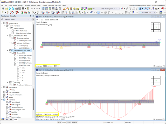
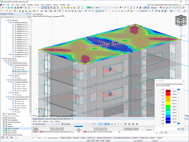
Odkształcenie prętów i powierzchni jest określane z uwzględnieniem zarysowanego (stan II) lub niezarysowanego (stan I) przekroju żelbetowego. Podczas określania sztywności można uwzględnić usztywnienie przy rozciąganiu między rysami, zwane 'usztywnieniem przy rozciąganiu', zgodnie z zastosowaną normą obliczeniową.
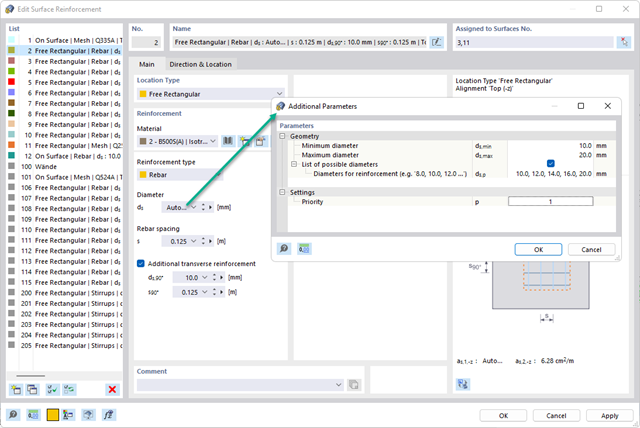
Istniejące zbrojenie powierzchniowe można automatycznie zaprojektować tak, aby pokryć wymagane zbrojenie. Można wybrać, czy automatycznie ma być definiowana średnica zbrojenia, czy też rozstaw prętów.
Przejdź do filmu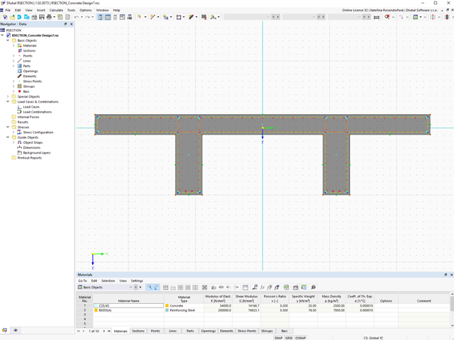
W rozszerzeniu Projektowanie konstrukcji betonowych można wymiarować dowolny przekrój RSECTION. Otulinę betonową, zbrojenie na ścinanie i zbrojenie podłużne definiuje się bezpośrednio w RSECTION.
Po zaimportowaniu przekroju ze zbrojeniem RSECTION do programu RFEM 6, można go również wykorzystać do obliczeń w rozszerzeniu Projektowanie konstrukcji betonowych.
Przejdź do filmu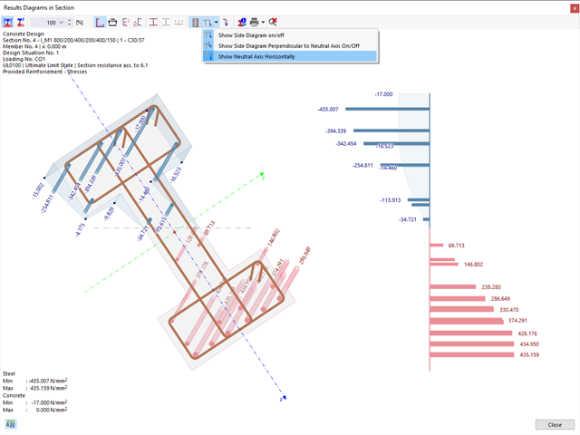
Istniejące naprężenia i odkształcenia przekroju betonowego i zbrojenia można wyświetlić w postaci obrazu naprężeń 3D lub grafiki 2D. W zależności od tego, które wyniki zostaną wybrane w drzewie wyników, naprężenia lub odkształcenia są wyświetlane w zdefiniowanym zbrojeniu podłużnym pod oddziaływaniami obciążeń lub granicznymi siłami wewnętrznymi.
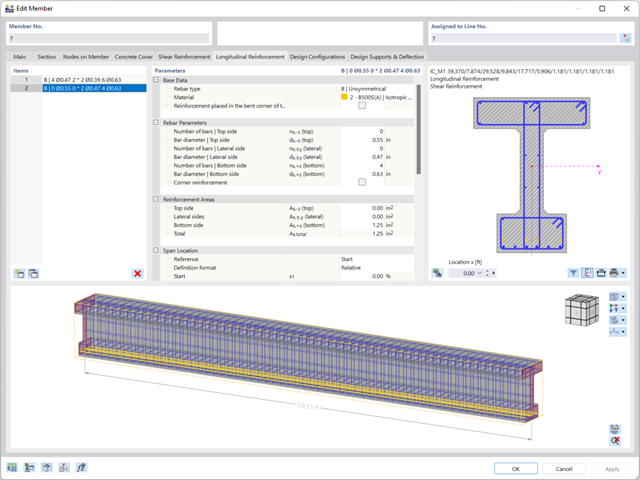
Zbrojenie na ścinanie i zbrojenie podłużne można zdefiniować indywidualnie dla każdego pręta. W tym przypadku dostępne są różne szablony do wprowadzania zbrojenia.
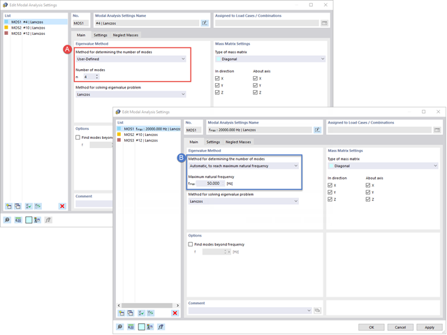
Twoim celem jest określenie liczby postaci drgań własnych? Program oferuje dwie metody. Z jednej strony, można ręcznie zdefiniować liczbę najmniejszych kształtów drgań, które mają zostać obliczone. W tym przypadku liczba dostępnych kształtów postaci zależy od stopni swobody (tzn. liczby punktów mas swobodnych pomnożonych przez liczbę kierunków, w których działają masy). Jest to jednak ograniczone do 9999. Z drugiej strony, maksymalną częstotliwość drgań własnych można ustawić w taki sposób, w jaki program określił kształty automatycznie, aż do osiągnięcia zadanej częstotliwości drgań własnych.
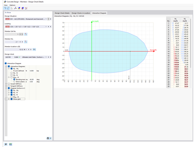
Czy chcesz określić nośność przekroju żelbetowego na zginanie dwukierunkowe? W tym celu należy najpierw aktywować wykres interakcji moment-moment (wykres My-Mz). Wykres My-Mz przedstawia poziomy przekrój przez trójwymiarowy wykres dla określonej siły osiowej N. Dzięki połączeniu z trójwymiarowym wykresem interakcji można tam również zwizualizować płaszczyznę przekroju.
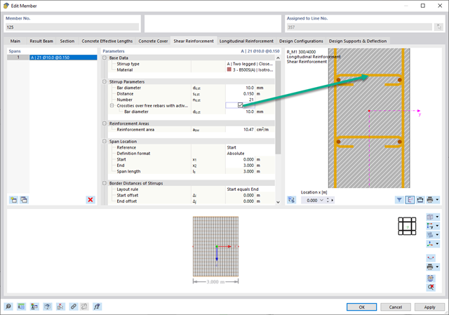
W zakładce "Zbrojenie na ścinanie" można wybrać opcję "Powiązania krzyżowe na wolnych prętach zbrojeniowych z aktywnym wyborem w oknie graficznym". Pozwala to na umieszczenie dodatkowych powiązań krzyżowych na wolnych prętach zbrojenia podłużnego.
Pozycję więzów krzyżowych można aktywować lub dezaktywować w infografice. Powiązania krzyżowe są uwzględniane podczas kontroli stanu granicznego nośności i obliczeń konstrukcji. Są one dostępne dla obliczeń zgodnie z EN 1992-1-1.
Przejdź do filmu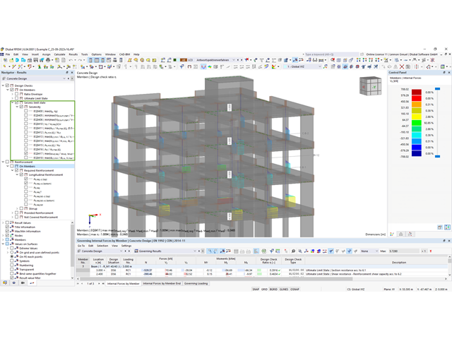
W rozszerzeniu Projektowanie konstrukcji betonowych można przeprowadzać obliczenia sejsmiczne dla prętów żelbetowych zgodnie z EC 8. Są to między innymi następujące funkcje:
- Konfiguracje obliczeń sejsmicznych
- Rozróżnianie klas ciągliwości DCL, DCM, DCH
- Możliwość przeniesienia współczynnika odpowiedzi z analizy dynamicznej
- Sprawdzenie wartości granicznej współczynnika odpowiedzi
- Weryfikacja nośności dla "Wytrzymały słup - słaba belka"
- Uszczegółowienie i reguły szczególne dla współczynnika ciągliwości krzywizny
- Uszczegółowienie i reguły szczególne dla ciągliwości lokalnej
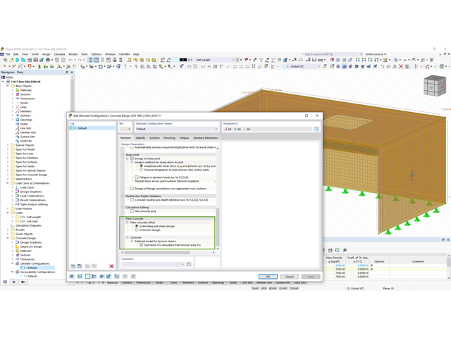
Teraz w rozszerzeniu Projektowanie konstrukcji betonowych można wymiarować elementy wykonane z betonu zbrojonego włóknami zgodnie z wytyczną "DAfStb Steel Fiber-Reinforced Concrete".
Ta opcja jest dostępna dla obliczeń zgodnie z EN 1992-1-1. Obliczenia zgodnie z wytyczną DAfStb są przeprowadzane po przypisaniu betonu typu "Fibrobeton" do elementu konstrukcyjnego z betonu zbrojonego.
Przejdź do filmu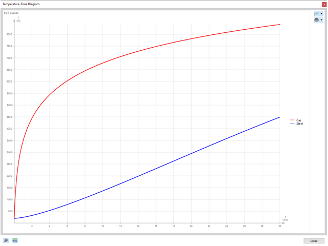
- 002327
- Ogólne informacje
- Projektowanie konstrukcji stalowych RFEM 6
- Projektowanie konstrukcji stalowych RSTAB 9
Na podstawie danych wejściowych można automatycznie określić decydującą temperaturę elementu w momencie przeprowadzania analizy. W takim przypadku można szczegółowo prześledzić krzywą temperatury w funkcji czasuwykres temperatura-czas.
.png?mw=640&hash=3c928fddb4215c3df06e0b731d5c3f2e475cd9db)
W ramach jednego pręta można zdefiniować szerokość integracyjną i efektywną szerokość płyty belek teowych (żeber) o różnych szerokościach. Pręt jest podzielony na segmenty. Przejście między różnymi szerokościami półek można sortować lub określać liniowo. Ponadto program umożliwia uwzględnienie zdefiniowanego zbrojenia powierzchni jako zbrojenia pasa przy wymiarowaniu żebra w betonie zbrojonym.
- 002557
- Ogólne informacje
- Projektowanie konstrukcji betonowych RFEM 6
- Projektowanie konstrukcji betonowych RSTAB 9
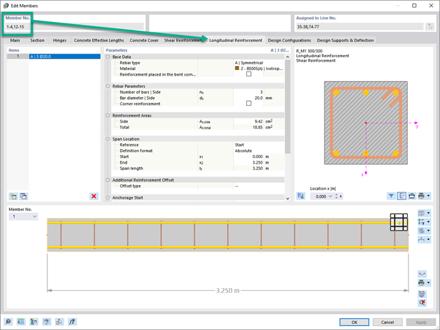
Skorzystaj i oszczędzaj czas! Ta funkcja umożliwia jednoczesne definiowanie lub edycję zbrojenia dla kilku prętów lub zbiorów prętów.
Przejdź do filmu- 002171
- Ogólne informacje
- Projektowanie konstrukcji stalowych RFEM 6
- Projektowanie konstrukcji stalowych RSTAB 9
W porównaniu z modułem dodatkowym RF-/STEEL EC3 (RFEM 5/RSTAB 8) do rozszerzenia Wymiarowanie stali dla programu RFEM 6/RSTAB 9 dodano następujące nowe funkcje:
- Oprócz Eurokodu 3, uwzględnione zostały inne międzynarodowe normy (np. AISC 360, CSA S16, GB 50017, SP 16.13330)
- Berücksichtigung der Feuerverzinkung (DASt-Richtlinie 027) beim Brandschutznachweis nach EN 1993-1-2
- Opcja wprowadzania żeber usztywniających, które można uwzględnić w analizie wyboczenia
- Wyboczenie skrętne można również sprawdzić w przypadku przekrojów zamkniętych (np. istotne dla smukłych, wysokich prostokątnych przekrojów zamkniętych)
- Automatyczne wykrywanie prętów lub zbiorów prętów ważnych dla obliczeń (np. automatyczna dezaktywacja prętów z nieaktualnym materiałem lub prętów już zawartych w zbiorze prętów)
- Możliwość dostosowania ustawień obliczeniowych indywidualnie dla każdego pręta
- Graficzne przedstawienie wyników w przekroju brutto lub przekroju efektywnym
- Wyświetlanie odpowiednich wzorów użytych do sprawdzania warunków nośności (w tym odniesienie do zastosowanego równania z normy)
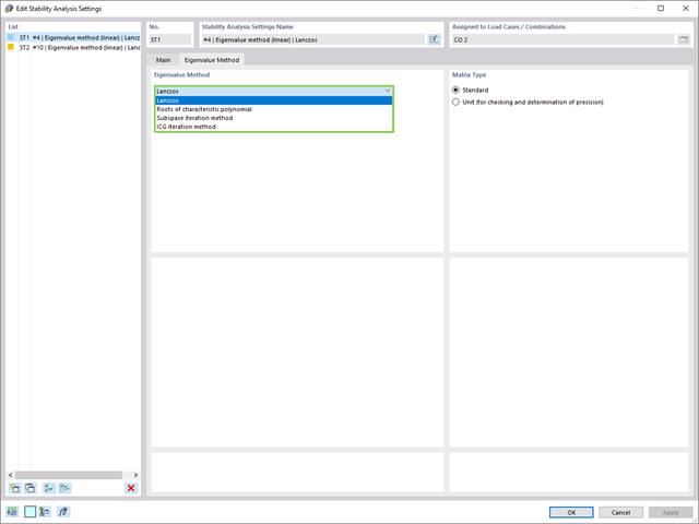
W przypadku analizy wartości własnych dostępnych jest kilka metod:
- Metody bezpośrednie
- Metody bezpośrednie (Lanczosa [RFEM], pierwiastki z wielomianu charakterystycznego [RFEM], metoda iteracji podprzestrzeni [RFEM/RSTAB], przesunięta iteracja odwrócona [RSTAB]) są odpowiednie dla małych i średnich modeli. Z szybkich metod rozwiązywania problemów należy korzystać tylko w przypadku, gdy komputer posiada dużą ilość pamięci RAM.
- Metoda iteracji ICG (niekompletny sprzężony gradient [RFEM])
- Z drugiej strony, ta metoda wymaga tylko niewielkiej ilości pamięci. Wartości własne są określane jedna po drugiej. Może być stosowany do obliczania dużych układów konstrukcyjnych o niewielkiej liczbie wartości własnych.
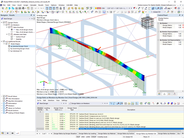
Rozszerzenie Stateczność konstrukcji umożliwia nieliniową analizę stateczności przy użyciu metody przyrostowej. Analiza ta dostarcza wyniki zbliżone do rzeczywistości również w przypadku konstrukcji nieliniowych. Współczynnik obciążenia krytycznego jest określany poprzez stopniowe zwiększanie obciążeń w podstawowym przypadku obciążenia, aż do osiągnięcia niestateczności. Przyrost obciążenia uwzględnia nieliniowości, takie jak ulegające uszkodzeniu pręty, podpory i fundamenty oraz nieliniowości materiałowe. Po zwiększeniu obciążenia można opcjonalnie przeprowadzić liniową analizę stateczności na ostatnim stabilnym stanie w celu określenia postaci stateczności.
- 002333
- Ogólne informacje
- Projektowanie konstrukcji stalowych RFEM 6
- Projektowanie konstrukcji stalowych RSTAB 9
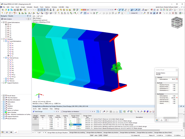
Rozszerzenie Skręcanie skrępowane (7 stopni swobody) oferuje szereg nowych opcji. W programach RFEM i RSTAB można na przykład przeprowadzić obliczenia konstrukcji prętowych z uwzględnieniem deplanacji przekroju. Wypadkowe siły wewnętrzne (N, Vu, Vv, Mt,pri, Mt,sec, Mu, Mv, Mω) można uwzględnić w analizie naprężeń równoważnych dla konstrukcji stalowych. Powiadomienia Funkcja ta nie jest obecnie dostępna dla norm projektowych AISC 360-16 i GB 50017.
- 002335
- Ogólne informacje
- Projektowanie konstrukcji stalowych RFEM 6
- Projektowanie konstrukcji stalowych RSTAB 9
Czy do określenia współczynnika obciążenia krytycznego do analizy stateczności użyto solwera wartości własnych rozszerzenia? W ten sposób można wyświetlić decydujący kształt drgań własnych projektowanego obiektu. Na potrzeby analizy zwichrzenia dostępny jest solwer wartości własnych, w zależności od zastosowanej normy obliczeniowej. W przypadku metody ogólnej zgodnie z EN 1993-1-1, 6.3.4 można również użyć wewnętrznego solwera wartości własnych.