338 Wyniki
Wyświetl wyniki:
Sortuj według:

W rozszerzeniu Projektowanie konstrukcji betonowych dla programu RFEM 6 można przeprowadzić obliczenia odporności ogniowej ścian i płyt żelbetowych zgodnie z uproszczoną metodą tabelaryczną (EN 1992-1-2, rozdział 5.4.2 oraz tabele 5.8 i 5.9).
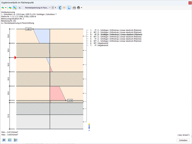
Istnieje możliwość wymiarowania powierzchni z uwagi na warunki pożarowe przy użyciu metody zredukowanego przekroju. Redukcja jest stosowana na grubości powierzchni. Kontrolę obliczeń można przeprowadzić dla wszystkich materiałów drewnianych, które są dopuszczone dla obliczeń.
W przypadku drewna klejonego krzyżowo, w zależności od rodzaju kleju, można wybrać, czy możliwe jest odpadanie poszczególnych zwęglonych części warstwy, a tym samym, czy można spodziewać się zwiększonego zwęglenia w niektórych obszarach warstwy.
- 002691
- Ogólne informacje
- Projektowanie konstrukcji betonowych RFEM 6
- Projektowanie konstrukcji betonowych RSTAB 9
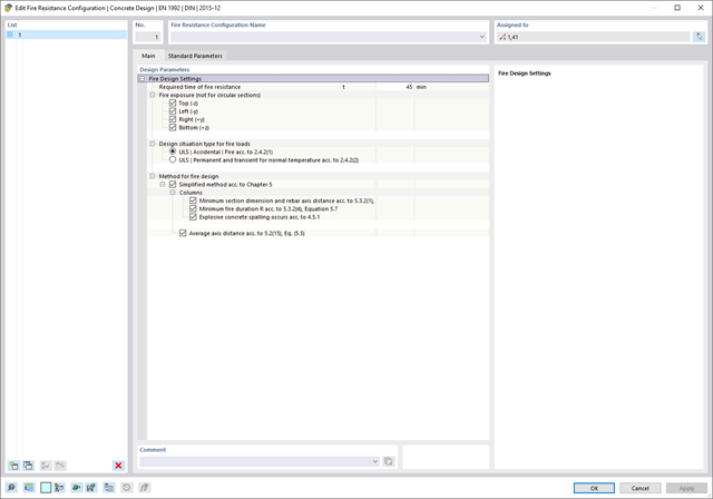
W rozszerzeniu Projektowanie konstrukcji betonowych można przeprowadzić uproszczone obliczenia odporności ogniowej słupów (Rozdział 5.3.2) i belek (Rozdział 5.6), zgodnie z EN 1992-1-2.
W przypadku uproszczonych obliczeń odporności ogniowej dostępne są następujące metody weryfikacji:
- Słupy: Minimalne wymiary przekroju prostokątnego i okrągłego wg tabeli 5.2a oraz równania 5.7 do obliczania czasu ekspozycji pożarowej
- Belki: Minimalne wymiary i odległości między środkami zgodnie z Tabelą 5.5 i Tabelą 5.6
Siły wewnętrzne do obliczeń odporności ogniowej można wyznaczyć przy użyciu dwóch metod.
- 1: W tym przypadku siły wewnętrzne z wyjątkowej sytuacji obliczeniowej są bezpośrednio uwzględniane w obliczeniach.
- 2: Siły wewnętrzne z obliczeń w temperaturze normalnej są redukowane za pomocą współczynnika Eta,fi (ηfi) i są następnie wykorzystywane do obliczeń odporności ogniowej.
Ponadto istnieje możliwość modyfikacji rozstawu osi zgodnie z równ. 5.5.
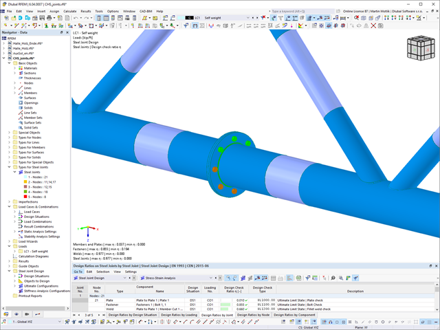
W rozszerzeniu Połączenia stalowe można łączyć profile zamknięte o przekroju okrągłym za pomocą spoin.
Profile okrągłe można łączyć ze sobą lub z płaskimi elementami konstrukcyjnymi. Spoiną można również łączyć pachwiny przekrojów znormalizowanych i cienkościennych.
Przejdź do filmu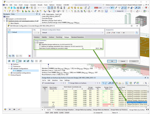
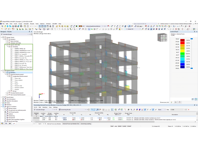
Rozszerzenie Projektowanie konstrukcji betonowych umożliwia wymiarowanie prętów i powierzchni ze względu na zmęczenie zgodnie z EN 1992-1-1, rozdział 6.8.
W przypadku obliczeń zmęczenia można opcjonalnie wybrać dwie metody lub poziomy obliczeniowe w konfiguracjach obliczeniowych:
- Poziom obliczeniowy 1: Obliczenia uproszczone wg. do 6.8.6 i 6.8.7(2) Kryterium uproszczone jest stosowane dla częstych kombinacji oddziaływań zgodnie z EN 1992-1-1, rozdział 6.8.6 (2) oraz EN 1990, równ. (6.15b) wraz z obciążeniami od ruchu drogowego w stanie użytkowalności. Dla stali zbrojeniowej sprawdzany jest maksymalny zakres naprężeń zgodnie z 6.8.6. Naprężenie ściskające w betonie jest określane za pomocą górnego i dolnego dopuszczalnego naprężenia zgodnie z 6.8.7(2).
- Poziom analizy 2: Obliczanie równoważnego naprężenia niszczącego zgodnie z 6.8.5 i 6.8.7(1) (uproszczone obliczenia na zmęczenie): Obliczenia z wykorzystaniem zakresów równoważnych naprężeń niszczących są przeprowadzane dla kombinacji zmęczeniowych, zgodnie z EN 1992-1-1, rozdział 6.8.3, równ. (6.69) o specyficznie zdefiniowanym oddziaływaniu cyklicznym Qfat .
W rozszerzeniu Projektowanie konstrukcji betonowych można przeprowadzać obliczenia sejsmiczne dla prętów żelbetowych zgodnie z EC 8. Są to między innymi następujące funkcje:
- Konfiguracje obliczeń sejsmicznych
- Rozróżnianie klas ciągliwości DCL, DCM, DCH
- Możliwość przeniesienia współczynnika odpowiedzi z analizy dynamicznej
- Sprawdzenie wartości granicznej współczynnika odpowiedzi
- Weryfikacja nośności dla "Wytrzymały słup - słaba belka"
- Uszczegółowienie i reguły szczególne dla współczynnika ciągliwości krzywizny
- Uszczegółowienie i reguły szczególne dla ciągliwości lokalnej
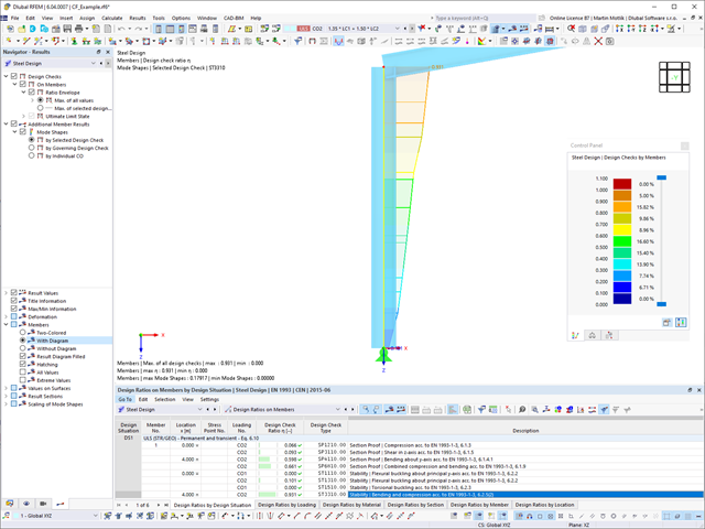
W rozszerzeniu Projektowanie konstrukcji stalowych można przeprowadzić kontrolę obliczeń stateczności i przekrojów profili formowanych na zimno według EN 1993-1-3, zgodnie z punktami 6.1.2 - 6.1.5 i 6.1.8 - 6.1.10.
Przejdź do filmu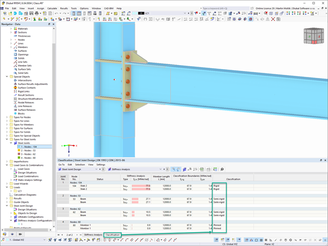
W rozszerzeniu Połączenia stalowe można klasyfikować sztywności połączeń.
Oprócz sztywności początkowej w tabeli wyświetlane są również wartości graniczne dla połączeń przegubowych i sztywnych dla wybranych sił wewnętrznych N, My i/lub Mz. Uzyskana klasyfikacja jest następnie wyświetlana w tabeli jako „przegubowa”, „półsztywna” i „sztywna”.
Przejdź do filmu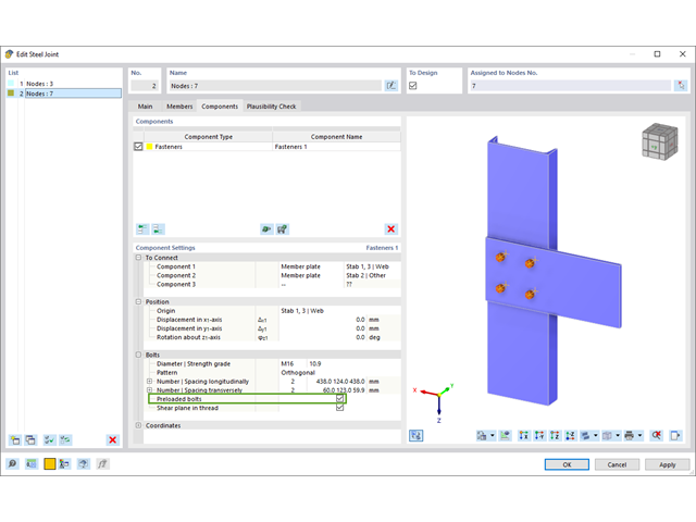
W rozszerzeniu „Połączenia stalowe” można uwzględnić naprężenie wstępne śrub w obliczeniach dla wszystkich komponentów. Sprężenie można łatwo aktywować za pomocą pola wyboru w parametrach śruby i ma ono wpływ zarówno na analizę naprężeniowo-odkształceniową, jak i na analizę sztywności.
Śruby sprężone to specjalne śruby stosowane w konstrukcjach stalowych w celu wygenerowania dużej siły zaciskowej między połączonymi elementami konstrukcyjnymi. Ta siła docisku powoduje tarcie między elementami konstrukcyjnymi, co umożliwia przenoszenie sił.
Funkcjonalność
Śruby sprężane są dokręcane z określonym momentem, co powoduje ich rozciąganie i powstawanie siły rozciągającej. Ta siła rozciągająca jest przenoszona na połączone elementy i prowadzi do powstania dużej siły mocującej. Siła zaciskowa zapobiega poluzowaniu połączenia i zapewnia niezawodne przenoszenie siły.
Zalety
- Wysoka nośność: Śruby wstępnie rozciągane mogą przenosić duże siły.
- Niskie odkształcenie: Minimalizują odkształcenie połączenia.
- Wytrzymałość zmęczeniowa: Są odporne na zmęczenie.
- Łatwość montażu: Są one stosunkowo łatwe w montażu i demontażu.
Analiza i wymiarowanie
Obliczenia śrub sprężanych są przeprowadzane w RFEM z wykorzystaniem modelu analitycznego ES wygenerowanego przez rozszerzenie "Połączenia stalowe". Uwzględnia ona siłę zwarcia, tarcie między elementami konstrukcyjnymi, wytrzymałość śrub na ścinanie oraz nośność elementów konstrukcyjnych. Wymiarowanie odbywa się zgodnie z DIN EN 1993-1-8 (Eurokod 3) lub amerykańską normą ANSI/AISC 360-16. Utworzony model analityczny wraz z wynikami można zapisać i wykorzystać jako niezależny model w programie RFEM.
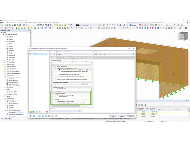
Teraz w rozszerzeniu Projektowanie konstrukcji betonowych można wymiarować elementy wykonane z betonu zbrojonego włóknami zgodnie z wytyczną "DAfStb Steel Fiber-Reinforced Concrete".
Ta opcja jest dostępna dla obliczeń zgodnie z EN 1992-1-1. Obliczenia zgodnie z wytyczną DAfStb są przeprowadzane po przypisaniu betonu typu "Fibrobeton" do elementu konstrukcyjnego z betonu zbrojonego.
Przejdź do filmu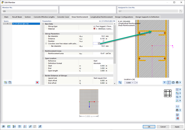
W zakładce "Zbrojenie na ścinanie" można wybrać opcję "Powiązania krzyżowe na wolnych prętach zbrojeniowych z aktywnym wyborem w oknie graficznym". Pozwala to na umieszczenie dodatkowych powiązań krzyżowych na wolnych prętach zbrojenia podłużnego.
Pozycję więzów krzyżowych można aktywować lub dezaktywować w infografice. Powiązania krzyżowe są uwzględniane podczas kontroli stanu granicznego nośności i obliczeń konstrukcji. Są one dostępne dla obliczeń zgodnie z EN 1992-1-1.
Przejdź do filmu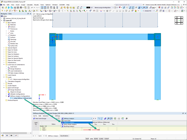
Sztywność początkowa Sj,ini jest parametrem decydującym o ocenie, czy połączenie można scharakteryzować jako sztywne, niesztywne czy przegubowe.
W rozszerzeniu „Połączenia stalowe” można obliczyć początkowe sztywności Sj,ini zgodnie z Eurokodem (EN 1993-1-8 sekcja 5.2.2) i AISC (AISC 360-16 Cl. E3.4) w odniesieniu do sił wewnętrznych N, My i/lub Mz.
Opcjonalne automatyczne przenoszenie sztywności początkowych umożliwia bezpośrednie przenoszenie sztywności przegubowych na końcach prętów w programie RFEM. Następnie cała konstrukcja jest ponownie obliczana, a wynikające z niej siły wewnętrzne są automatycznie uwzględniane jako obciążenia w obliczeniach i wymiarowaniu modeli połączeń.
Ten zautomatyzowany proces iteracji eliminuje konieczność ręcznego eksportu i importu danych, zmniejszając ilość pracy i minimalizując potencjalne źródła błędów.
Film wyjaśniający: Obliczanie sztywności początkowej Sj,ini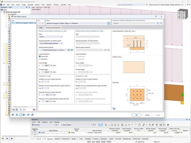
Czy wiecie, że...? W podporach obliczeniowych można teraz zdefiniować śruby z pełnym gwintem jako poprzeczne elementy wzmacniające ściskanie dla obliczenia "Ściskania w poprzek włókien". Śruby są sprawdzane pod kątem wciśnięcia i wyboczenia.
Dodatkowo sprawdzana jest nośność na ścinanie w płaszczyźnie wierzchołka śruby. Kąt rozłożenia obciążenia można uwzględnić liniowo poniżej 45° lub nieliniowo (zgodnie z Bejtka, I. (2005). Verstärkung von Bauteilen aus holz mit vollgewindeschrauben. KIT Scientific Publishing.
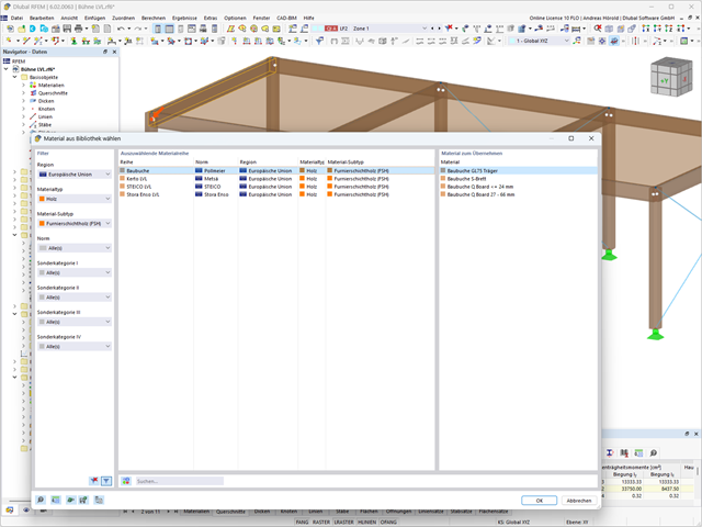
W programach RFEM i RSTAB można wymiarować pręty przy użyciu materiału typu "Fornir klejony warstwowo". Dostępni są następujący producenci:
- Pollmeier (Baubuche)
- Metsä (kerto LVL)
- STEICO
- Stora Enso
W konfiguracji stanu granicznego nośności można uwzględnić współczynniki wytrzymałości w celu zwiększenia wytrzymałości. Niezależnie od tego współczynniki zmniejszające wytrzymałości są uwzględniane automatycznie. Wypróbuj teraz!
Przejdź do filmu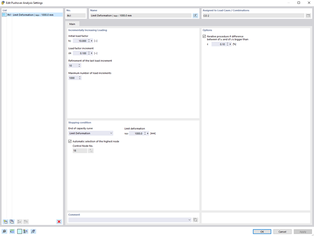
Analiza pushover jest zarządzana przez nowo wprowadzony typ analizy w kombinacjach obciążeń. W tym miejscu można wybrać poziomy rozkład i kierunek obciążenia, obciążenie stałe, żądane spektrum odpowiedzi do określenia docelowego przemieszczenia oraz ustawienia analizy pushover.
W ustawieniach analizy pushover można zmodyfikować przyrost obciążenia poziomego i określić warunek zatrzymania dla analizy. Ponadto użytkownik może bez problemu dostosować precyzyjność iteracyjnego definiowania przesunięcia docelowego.
- Uwzględnienie nieliniowego zachowania komponentu przy użyciu standardowych przegubów plastycznych dla stali (FEMA 356, EN 1998-3) i nieliniowego zachowania materiału (mur, stal - bilinearnie, krzywe robocze zdefiniowane przez użytkownika)
- Bezpośredni import mas z przypadków obciążeń lub kombinacji w celu przyłożenia stałych obciążeń pionowych
- Zdefiniowane przez użytkownika specyfikacje dotyczące uwzględniania obciążeń poziomych (ujednoliconych ze względu na postać drgań lub równomiernie rozłożonych na wysokości mas)
- Wyznaczanie krzywej pushover z możliwością wyboru kryterium granicznego obliczeń (zawalenie lub odkształcenie graniczne)
- Transformacja krzywej pushover w spektrum nośności (format ADRS, układ o jednym stopniu swobody)
- Bilinearyzacja spektrum nośności zgodnie z EN 1998-1:2010 + A1:2013
- Transformacja zastosowanego spektrum odpowiedzi w wymagane spektrum (format ADRS)
- Wyznaczanie docelowego przemieszczenia zgodnie z EC 8 (metoda N2 zgodnie z Fajfar 2000)
- Graficzne porównanie nośności i wymaganego spektrum
- Graficzna ocena kryteriów akceptacji zdefiniowanych przegubów plastycznych
- Wyświetlanie wyników obliczeń iteracyjnych docelowego przemieszczenia
- Dostęp do wszystkich wyników analizy statyczno-wytrzymałościowej w poszczególnych poziomach obciążenia
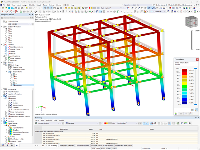
Podczas obliczeń wybrane obciążenie poziome jest zwiększane w krokach obciążenia. Statyczna analiza nieliniowa jest przeprowadzana dla każdego kroku obciążenia, aż do osiągnięcia określonego warunku granicznego.
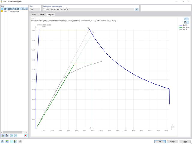
Wyniki analizy pushover są obszerne. Z jednej strony konstrukcja jest analizowana pod kątem odkstałceń. Można to przedstawić za pomocą linii siła-odkształcenie układu (krzywa nośności). Z drugiej strony, wpływ spektrum odpowiedzi można wyświetlić w oknie ADRS (Acceleration-Displacement Response Spectrum). Docelowe przemieszczenie jest określane w programie automatycznie na podstawie tych dwóch wyników. Proces można ocenić graficznie oraz w tabelach.
Poszczególne kryteria akceptacji można następnie przeanalizować i ocenić graficznie (dla następnego kroku obciążenia docelowego przemieszczenia, ale także dla wszystkich innych kroków obciążenia). Wyniki analizy statycznej są również dostępne dla poszczególnych kroków obciążenia.
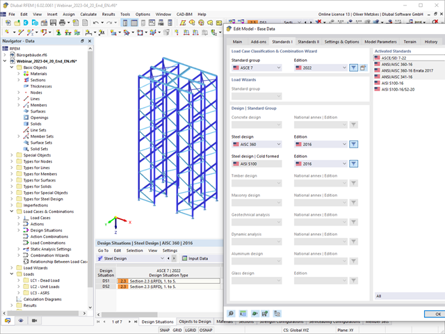
Wymiarowanie prętów stalowych formowanych na zimno zgodnie z AISI S100-16/CSA S136-16 jest dostępne w RFEM 6. Dostęp do obliczeń można uzyskać, wybierając normy „AISC 360” lub „CSA S16” w rozszerzeniu Projektowanie konstrukcji stalowych. Następnie dla obliczeń elementów formowanych na zimno automatycznie wybierane jest „AISI S100” lub „CSA S136”.
Do obliczania sprężystego obciążenia wyboczeniowego pręta program RFEM stosuje metodę DSM. Bezpośrednia metoda wytrzymałości oferuje dwa typy rozwiązań, numeryczne (metoda pasm skończonych) i analityczne (specyfikacja). Krzywą charakterystyczną (sygnaturę) FSM i kształty wyboczenia można wyświetlić w oknie dialogowym Przekroje.
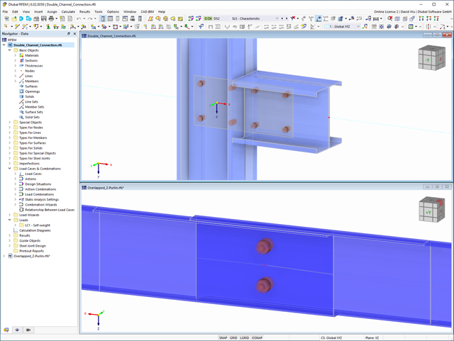
Rozszerzenie Połączenia stalowe umożliwia wymiarowanie połączeń prętów o złożonych przekrojach. Ponadto można przeprowadzać obliczenia połączeń dla prawie wszystkich przekrojów cienkościennych z biblioteki programu RFEM.
Przejdź do filmu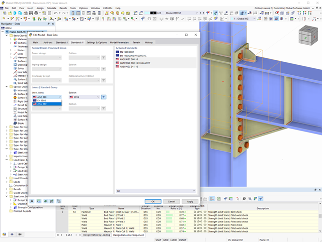
W rozszerzeniu Połączenia stalowe można wymiarować połączenia zgodnie z amerykańską normą ANSI/AISC 360-16. Zintegrowane zostały następujące metody obliczeń:
- Obliczenia współczynnika obciążenia i odporności (LRFD)
- Projektowanie dopuszczalnych naprężeń (ASD)
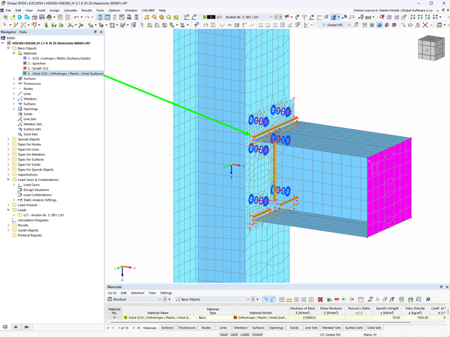
W tym przypadku projektowanie spoin staje się dziecinnie proste. Dzięki specjalnie opracowanemu modelowi materiałowemu „Ortotropowy | Plastyczny | Spoina (Powierzchnie)" można obliczyć wszystkie składowe naprężenia w sposób plastyczny. Naprężenie Tprostopadłe jest również rozpatrywane w sposób plastyczny.
Korzystanie z tego modelu materiałowego umożliwia realistyczne i ekonomiczne projektowanie spoin.
Film wyjaśniający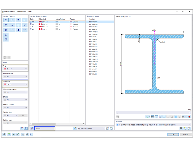
- 002567
- Ogólne informacje
- Projektowanie konstrukcji stalowych RFEM 6
- Projektowanie konstrukcji stalowych RSTAB 9
Nowe przekroje stalowe zgodnie z najnowszą instrukcją CISC (12 wydanie) są dostępne w programie RFEM 6. Przekroje są wymienione w bibliotece Znormalizowane. W filtrze należy wybrać region „Kanada”, a normę „CISC 12”. Alternatywnie nazwę przekroju można wprowadzić bezpośrednio w polu wyszukiwania znajdującym się w dolnej części okna dialogowego.
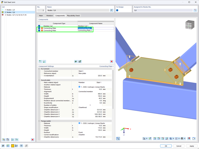
Za pomocą komponentu "Blacha łącząca" można automatycznie utworzyć nową blachę węzłową w rozszerzeniu Połączenia stalowe. Pozwala to na zaoszczędzenie oddzielnych komponentów, a pozostałe elementy, takie jak blacha czołowa i blacha nakładkowa, są automatycznie uwzględniane wraz z wymiarami.
Przejdź do filmu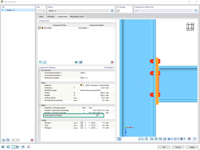
Aby określić nośność śrub na ścinanie, w rozszerzeniu Połączenia stalowe można określić, czy w połączeniu na ścinanie znajduje się trzpień czy gwint.
Przejdź do filmu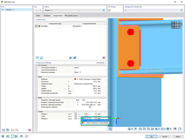
W przypadku spoiny łączącej dwie płyty z różnych materiałów, można teraz wybrać z pola rozwijanego, który z obu materiałów ma zostać użyty do utworzenia spoiny.
Przejdź do filmu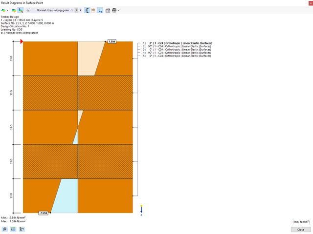
Rozszerzenie Projektowanie konstrukcji drewnianych dla RFEM umożliwia wymiarowanie prętów i powierzchni zgodnie z Eurokodem 5, SIA 265 (norma szwajcarska), CSA O86 (norma kanadyjska) lub ANSI/AWC NDS (norma amerykańska), np. drewno klejone krzyżowo, drewno klejone warstwowo, drewno iglaste, materiały drewnopochodne itp.
Przejdź do filmu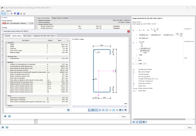
Chcesz przeprowadzić kontrolę przekrojów prętów stalowych zimnogiętych zgodnie z EN 1993-1-3? Niezależnie od tego, czy są to profile zimnogięte z biblioteki przekrojów, czy też przekroje ogólne formowane na zimno (nieperforowane) z RSECTION, program do analizy statyczno-wytrzymałościowej pomoże w definiowaniu przekroju efektywnego z uwzględnieniem wyboczenia lokalnego i niestateczności. Można również przeprowadzić kontrolę przekroju zgodnie z EN 19 93 1 3, sekcja 6 1 6. W takim przypadku siły wewnętrzne z obliczeń z wykorzystaniem Skręcania skrępowanego (7 stopni swobody) są uwzględniane za pomocą kontroli naprężeń zastępczych
Przejdź do filmu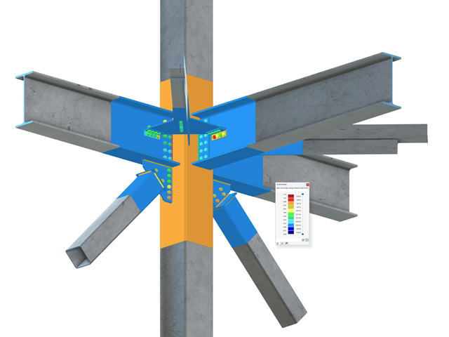
Złożone połączenie belek poziomych ze słupem oraz połączenie stężeń ukośnych
Model połączenia został zamodelowany przy użyciu około 50 komponentów. Model został stworzony na podstawie rzeczywistego przykładu wykorzystania w konstrukcji.
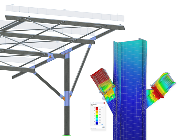
Stalowe połączenia śrubowe z blachami węzłowymi na konstrukcji zadaszenia.
Pobierz model do analizy statyczno-wytrzymałościowej i otwórz go w programie RFEM 6, korzystając z rozszerzenia Połączenia stalowe.
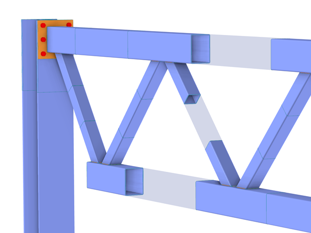
W przypadku przekrojów prostokątnych zwykle można uzyskać bezpośrednie połączenie za pomocą spoin. W ten sam sposób można je jednak połączyć z innymi przekrojami. Ponadto inne elementy, takie jak blachy czołowe, pomagają w łączeniu przekrojów prostokątnych z innymi elementami konstrukcyjnymi.