Online Manuals RFEM 6 | Multilayer Surfaces

Back to Online Manuals

2262x

003626

Dipl.-Ing. (FH) Bastian Kuhn, M.Sc.

2023-10-19

Select Manual

Overview

Multilayer Surfaces Add-on

Theory

Input

Results

Calculation Examples

Stiffnesses for Multilayer Surfaces

Material Models

Material models form the basis for combining multilayer surfaces to achieve efficient surface stiffness. Using the Multilayer Surfaces add-on, you can freely combine material models in RFEM 6. The fundamentals of material models are described in the chapters Materials and Nonlinear Material Behavior of the RFEM manual.

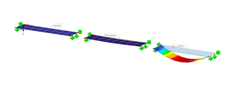
A selection of possible combinations of material models is created in the “Multilayer Models” model (see the right column), which you can download for further study of the combinations.

The following list shows a selection of possible combinations:

Isotropic layers (for example, concrete – steel)
Orthotropic layers (for example, cross-laminated timber)
Isotropic – orthotropic (for example, steel – GFRP)
Isotropic plastic – isotropic (for example, concrete – steel)
Isotropic nonlinear elastic – orthotropic (for example, concrete – timber)
Isotropic – orthotropic plastic (for example, concrete – timber)
Isotropic damage – orthotropic (for example, concrete – timber)

To combine nonlinear materials, it is necessary to activate the Nonlinear Material Behavior add-on.

Stiffnesses for Multilayer Surfaces Without Solids

The simpler calculation option in the Multilayer Surfaces add-on is to define different surface layers in the “Layers” thickness type without solids. However, the material models can also be freely combined here.

Once the layers have been defined, the Multilayer Surfaces add-on generates a global stiffness matrix for the surface. In RFEM, internal forces and deformations are calculated for this surface. In the respective design add-on, such as Timber Design or Stress-Strain analysis, these internal forces are then distributed among the existing layers. Usually, the internal forces are output at three integration points per location.

Calculation Process for Multilayer Surfaces

The following section explains the calculation of the stiffness matrix for isotropic and orthotropic materials.

Calculation of Stiffness Matrix

The following conditions apply as the basis for the material models (see the chapter Materials of the RFEM manual):

All stiffness values ≥ 0
Total stiffness matrix of surface must be positive definite.
Basic equation isotropic:

E = 2 G (1 + ν)

E	Modulus of elasticity
G	Shear modulus
ν	Poisson's ratio

Modulus of Elasticity, Shear Modulus, and Poisson's Ratio

Basic equation orthotropic:

\frac{ν_{y x}}{E_{y}} = \frac{ν_{x y}}{E_{x}}

Transversal Strain Relation

Local Stiffness Matrix by Layer

Isotropic

d_{i}' = [\begin{matrix} d'_{11, i} & d'_{12, i} & 0 \\ d'_{22, i} & 0 \\ s y m . & d'_{33, i} \end{matrix}] = [\begin{matrix} \frac{E_{i}}{1 - ν_{i}^{2}} & \frac{ν_{i} E_{i}}{1 - ν_{i}^{2}} & 0 \\ \frac{E_{i}}{1 - ν_{i}^{2}} & 0 \\ s y m . & G_{i} \end{matrix}] i = 1, . . ., n w h e r e G_{i} = \frac{E_{i}}{2 (1 + ν_{i})}

Stiffness Matrix for Isotropic Layer

Orthotropic

d_{i}' = [\begin{matrix} d'_{11, i} & d'_{12, i} & 0 \\ d'_{22, i} & 0 \\ s y m . & d'_{33, i} \end{matrix}] = [\begin{matrix} \frac{E_{x, i}}{1 - ν_{x y, i}^{2} \frac{E_{y, i}}{E_{x, i}}} & \frac{ν_{x y, i} E_{y, i}}{1 - ν_{x y, i}^{2} \frac{E_{y, i}}{E_{x, i}}} & 0 \\ \frac{E_{y, i}}{1 - ν_{x y, i}^{2} \frac{E_{y, i}}{E_{x, i}}} & 0 \\ s y m . & G_{x y, i} \end{matrix}] i = 1, . . ., n

Stiffness Matrix for Orthotropic Layer

Info

For orthotropic material, the in-plane shear modulus (G_xy) is defined by the material properties, while for isotropic material, it is determined from the modulus of elasticity and the Poisson's ratio. Therefore, the Poisson's ratio with the "location-cause" principle is important for the orthotropic material.

The shear stiffnesses for orthotropic material are as follows:

G_xy	In-plane shear modulus (for example, 690 N/mm² for C24)
G_xz	Shear modulus in the direction x over the thickness (for example, 690 N/mm² for C24)
G_yz	Shear modulus in the direction y over the thickness (for example, 690 N/mm² for C24) – also called "rolling shear modulus".

The special feature of orthotropic material is that directional stiffnesses can be defined in a surface. Usually, the local orientation of the surface or layer in the x-direction corresponds to the stiffness in the x-direction. However, since this can be freely defined via the angle β in the “Layers” thickness type, it is necessary to transform the stiffnesses accordingly.

d_{i} = [\begin{matrix} d_{11, i} & d_{12, i} & d_{13, i} \\ d_{22, i} & d_{23, i} \\ s y m . & d_{33, i} \end{matrix}] = T_{3 x 3, i}^{T} d'_{i} T_{3 x 3, i}

Transformation Stiffnesses

T_{3 x 3, i} = [\begin{matrix} c ² & s ² & c s \\ s ² & c ² & - c s \\ - 2 c s & 2 c s & c ² - s ² \end{matrix}] w h e r e c = \cos (β_{i}), s = \sin (β_{i})

Transformation Matrix

Summed element by layer:

d_{11, i} = c^{4} d'_{11, i} + 2 c ² s ² d'_{12, i} + s^{4} d'_{22, i} + 4 c ² s ² d'_{33, i}

d_{12, i} = c^{2} s^{2} d'_{11, i} + s^{4} d'_{12, i} + c^{4} d'_{12, i} + c ² s ² d'_{22, i} - 4 c ² s ² d'_{33, i}

d_{13, i} = c^{3} s d'_{11, i} + c s^{3} d'_{12, i} - c^{3} s d'_{12, i} - c s^{3} d'_{22, i} - 2 c^{3} s d'_{33, i} + 2 c s^{3} d'_{33, i}

d_{22, i} = s^{4} d'_{11, i} + 2 c ² s ² d'_{12, i} + c^{4} d'_{22, i} + 4 c ² s ² d'_{33, i}

d_{23, i} = c s^{3} d'_{11, i} + c^{3} s d'_{12, i} - c s^{3} d'_{12, i} - c^{3} s d'_{22, i} + 2 c^{3} s d'_{33, i} - 2 c s^{3} d'_{33, i}

d_{33, i} = c^{2} s^{2} d'_{11, i} - 2 c ² s ² d'_{12, i} + c^{2} s^{2} d'_{22, i} + {(c^{2} - s^{2})}^{2} d'_{33, i}

Individual Terms by Layer

Bending and Torsional Elements [Nm]

The matrix elements for bending and torsion are given in the following equations.

D_{11} = \sum_{i = 1}^{n} \frac{z_{m a x, i}^{3} - z_{m i n, i}^{3}}{3} d_{11, i}

Bending Stiffness in x

D_{12} = \sum_{i = 1}^{n} \frac{z_{m a x, i}^{3} - z_{m i n, i}^{3}}{3} d_{12, i}

Eccentricity Term (12)

D_{22} = \sum_{i = 1}^{n} \frac{z_{m a x, i}^{3} - z_{m i n, i}^{3}}{3} d_{22, i}

Bending Stiffness in y

D_{13} = \sum_{i = 1}^{n} \frac{z_{m a x, i}^{3} - z_{m i n, i}^{3}}{3} d_{13, i}

Eccentricity Term (13)

D_{23} = \sum_{i = 1}^{n} \frac{z_{m a x, i}^{3} - z_{m i n, i}^{3}}{3} d_{23, i}

Eccentricity Term (23)

D_{33} = \sum_{i = 1}^{n} \frac{z_{m a x, i}^{3} - z_{m i n, i}^{3}}{3} d_{33, i}

Torsional Stiffness

If there is only one layer in the “Layers” thickness type, the calculation is performed using the equations described in the RFEM manual.

For shear (elements D44/55), different equations apply in the “Layers” thickness type. They are described in the chapter Shear in Plate Plane.

Eccentricity Terms [Nm/m]

Asymmetrical panels result in eccentricity terms. An asymmetrical surface can occur, for example, in fire resistance calculations due to one-sided charring of a cross-laminated timber panel. The matrix elements are as follows:

D_{16} = \sum_{i = 1}^{n} \frac{z_{m a x, i}^{2} - z_{m i n, i}^{2}}{2} d_{11, i}

Eccentricity Element D16

D_{17} = \sum_{i = 1}^{n} \frac{z_{m a x, i}^{2} - z_{m i n, i}^{2}}{2} d_{12, i}

Eccentricity Element D17

D_{18} = \sum_{i = 1}^{n} \frac{z_{m a x, i}^{2} - z_{m i n, i}^{2}}{2} d_{13, i}

Eccentricity Element D18

D_{27} = \sum_{i = 1}^{n} \frac{z_{m a x, i}^{2} - z_{m i n, i}^{2}}{2} d_{22, i}

Eccentricity Element D27

D_{28} = \sum_{i = 1}^{n} \frac{z_{m a x, i}^{2} - z_{m i n, i}^{2}}{2} d_{23, i}

Eccentricity Element D28

D_{38} = \sum_{i = 1}^{n} \frac{z_{m a x, i}^{2} - z_{m i n, i}^{2}}{2} d_{33, i}

Eccentricity Element D38

Panel Plane [N/m]

The normal stiffnesses in the panel plane are handled in the plane of the panel. The D88 element is used to calculate the panel shear—that is, the shear force in the panel. The matrix elements are as follows:

D_{66} = \sum_{i = 1}^{n} t_{i} d_{11, i}

Normal Stiffness x D66

D_{67} = \sum_{i = 1}^{n} t_{i} d_{12, i}

Normal Stiffness Eccentric D67

D_{68} = \sum_{i = 1}^{n} t_{i} d_{13, i}

Normal Stiffness Eccentric D68

D_{77} = \sum_{i = 1}^{n} t_{i} d_{22, i}

Normal Stiffness y D77

D_{78} = \sum_{i = 1}^{n} t_{i} d_{23, i}

Normal Stiffness Eccentric D78

D_{88} = \sum_{i = 1}^{n} t_{i} d_{33, i}

Plate Shear D88

Shear in Panel Plane [N/m]

To determine the shear stiffness of an orthotropic material, it is necessary to rotate the stiffnesses according to their orientation relative to the local surface axis. This has to be done for each location of the “Layers” thickness type. In a simple composition with 0° orientation of the top layer and 90° orientation of the underlying layer, there is high shear compliance, which is it is necessary to take into account in the multi-layer model. This can be seen in the following image (source [1]) using the example of a cross-laminated timber panel.

Illustration of shear deformation in cross-laminated timber, provided by Informationsdienst Holz.

Shear Deformation (Source: Holzbau Deutschland | Informationsdienst Holz)

In laminate theory, the shear stiffness of a layer structure is calculated by transforming all bending and shear components into the respective directions of each layer. For more information on this topic, please refer to the reference list below.

Visualization of the alignment of stiffness axes in a laminate to optimize material properties.

Stiffness Orientation

The stiffnesses are summed up using the stiffness transformation displayed in the image. This summation is also known as the “Grashoff integral”.

D_{44, c a l c}^{"} = \frac{1}{\int_{- t / 2}^{t / 2} \frac{G_{22}^{"} (z)}{G_{11}^{"} (z) G_{22}^{"} (z) - {G_{12}^{"}}^{2} (z)} {(\frac{\int_{z}^{t / 2} E_{x}^{"} (\bar{z}) (\bar{z} - z_{0, x}) d \bar{z}}{\int_{- t / 2}^{t / 2} E_{x}^{"} (\bar{z}) {(\bar{z} - z_{0, x})}^{2} d \bar{z}})}^{2} d z}

Shear Stiffness in x-Direction

To calculate stiffness in the x- and y-direction, a center of stiffness is calculated for each multilayer surface structure.

z_{0, x} = \frac{\int_{- t / 2}^{t / 2} E_{x}^{"} (z) z d z}{\int_{- t / 2}^{t / 2} E_{x}^{"} (z) d z} = \frac{I_{1}}{I_{0}}

Center of Stiffness in x

D_{55, c a l c}^{"} = \frac{1}{\int_{- t / 2}^{t / 2} \frac{G_{11}^{"} (z)}{G_{11}^{"} (z) G_{22}^{"} (z) - {G_{12}^{"}}^{2} (z)} {(\frac{\int_{z}^{t / 2} E_{y}^{"} (\bar{z}) (\bar{z} - z_{0, x}) d \bar{z}}{\int_{- t / 2}^{t / 2} E_{y}^{"} (\bar{z}) {(\bar{z} - z_{0, x})}^{2} d \bar{z}})}^{2} d z}

Shear Rigidity in y-Direction

Center of stiffness in the y-direction:

z_{0, x} = \frac{\int_{- t / 2}^{t / 2} E_{y}^{"} (z) z d z}{\int_{- t / 2}^{t / 2} E_{y}^{"} (z) d z} = \frac{I_{1}}{I_{0}}

Center of Stiffness in y-Direction

In order to capture the orientation by location in the calculation of shear stiffness, the stiffnesses are determined according to the following equations.

G_{11, i}^{"} = \cos^{2} (φ - ß_{i}) G_{x z, i} + \sin^{2} (φ - ß_{i}) G_{y z, i}

Oriented Shear Stiffness G11

G stands for the shear stiffness of the layers in order to avoid confusion with the elements of the stiffness matrix (D).

The shear stiffness by layer can also be displayed in the matrix form as follows:

[\begin{matrix} G_{11} & G_{12} \\ G_{21} & G_{22} \end{matrix}]

Shear Stiffness Matrix

G_{22, i}^{"} = \sin^{2} (φ - ß_{i}) G_{x z, i} + \cos^{2} (φ - ß_{i}) G_{y z, i}

Oriented Shear Stiffness G22

The eccentric shear stiffness in the following equation would always be zero for the symmetrical structure of cross-laminated timber (0°/90°/0°) mentioned at the beginning and would therefore not be relevant. However, in the case of diagonal laminated timber (DLT), for example, this eccentricity member is not zero and therefore plays an important role.

G_{12}^{"} = (G_{x z, i} - G_{y z, i}) \sin (φ - ß_{i}) \cos (φ - ß_{i})

Eccentric Oriented Shear Stiffness G12

Further information can be found in [4] and in this YouTube video, among others.

Calculation of Shear Stiffness

The shear stiffness is determined in the following steps:

First, the angle of maximum stiffness is determined. The angle φ shows the change in the local coordinate system x of the surface to the oriented direction x.

All stiffnesses are rotated in the oriented direction x’' according to the equations presented above.

The panel stiffness matrix of each layer (3 x 3) is transformed from the local coordinate system x', y' into the rotated system x, y". In addition to the calculation of the directional shear stiffness of each individual layer, this is also done for the elastic moduli of each layer.

$E_{x, i}^{"} = d_{12, i}^{"} + \frac{2 d_{12, i}^{"} d_{13, i}^{"} d_{23, i}^{"} - d_{22, i}^{"} {(d_{13, i}^{"})}^{2} - d_{33, i}^{"} {(d_{12, i}^{"})}^{2}}{d_{22, i}^{"} d_{33, i}^{"} - {(d_{23, i}^{"})}^{2}}$

Oriented Modulus of Elasticity in x-Direction

$E_{y, i}^{"} = d_{22, i}^{"} + \frac{2 d_{12, i}^{"} d_{13, i}^{"} d_{23, i}^{"} - d_{11, i}^{"} {(d_{23, i}^{"})}^{2} - d_{33, i}^{"} {(d_{12, i}^{"})}^{2}}{d_{11, i}^{"} d_{33, i}^{"} - {(d_{13, i}^{"})}^{2}}$

Oriented Modulus of Elasticity in y-Direction

The shear stiffness is calculated using the equations described above (Grashoff integral). The shear stiffness is calculated using the individual components.

$I = \int_{- h / 2}^{h / 2} d_{11} (z) {(z - z_{0, x})}^{2} d z = \sum_{i = 1}^{n} d_{11, i} \frac{{(z_{m a x, i} - z_{0, x})}^{3} - {(z_{m i n, i} - z_{0, x})}^{3}}{3}$

Second Moment of Area in x-Direction

$χ_{i} = d_{11, i} \frac{{(z_{m a x, i} - z_{0, x})}^{2}}{2} + \sum_{k = i + 1}^{n} d_{11, k} \frac{{(z_{m a x, i} - z_{0, x})}^{2} - {(z_{m i n, i} - z_{0, x})}^{2}}{2}$

Equivalent Stiffness by Layer (in x)

Here, the equations are shown only for the x-direction (D44). The same applies to the y-direction. The equivalent stiffness (Steiner component) is calculated for each location.

The calculated stiffnesses for the oriented direction of an overall structure are finally calculated back via the angular relation and shown as original stiffnesses D44, D55, and D45 in the stiffness matrix.

$D_{44} = \cos^{2} (φ) D_{44}^{"} + \sin^{2} (φ) D_{55}^{"}$

Recalculated Shear Stiffness D44

$D_{55} = \sin^{2} (φ) D_{44}^{"} + \cos^{2} (φ) D_{55}^{"}$

Recalculated Shear Stiffness D55

$D_{45} = \sin (φ) \cos (φ) (D_{44}^{"} - D_{55}^{"})$

Recalculated Shear Stiffness D45

Increasing Shear Stiffness

Since modeling laminates as surfaces also allows for geometries with very narrow surface strips, it is necessary to increase the shear stiffness accordingly when calculating such problematic geometries.

This is displayed for the X-direction in the following equation

$D_{44}^{"} = \max (D_{44, calc}^{"}, \frac{48}{5 l ²} \frac{1}{\frac{1}{\sum_{i = 1}^{n} E_{x, i}^{"} \frac{t_{i}^{3}}{12}} - \frac{1}{\sum_{i = 1}^{n} E_{x, i}^{"} \frac{z_{\max, i}^{3} - z_{\min, i}^{3}}{3}}})$

Maximum Shear Stiffness

The length l in the above equation refers to the shortest length of a box that can be placed over the corresponding geometry.

In another model, which can be downloaded on the right-hand side, a narrow surface with a width of 10 cm was compared with an identical surface with a width of 20 cm.

The shear stiffness of the narrow surface is D44 = 15,253 kN/m compared to D44 = 5,970.8 kN/m for the wider surface. As a result, despite identical loading, the deformation of the stiffer surface is lower and the shear load is greater.

Stiffnesses for Multilayer Surfaces with Integrated Solids

In the future, it will also be possible to define solids together with surfaces in the Multilayer Surfaces add-on. With this type, a surface is also exported to RFEM. Since the generation of stiffnesses and the decomposition of internal forces is more complex, this will be explained separately.

References

Informationsdienst Holz. (2016). Bauen mit Brettsperrholz Tragende Massivholzelemente für Wand, Decke und Dach (Ser. 4, Part 6, Ep. 1). Berlin, Informationsdienst Holz.

Altenbach, H., Altenbach, J., & Naumenko, K. (2023). Ebene Flächentragwerke: Grundlagen der Modellierung und Berechnung von Scheiben und Platten. Berlin, Springer Vieweg.

Jones, R. M. (n.d.). Mechanics of Composite Materials (2nd ed.). Taylor & Francis Inc., Philadelphia.

Arnold, M. (2024). Mechanical Properties of Diagonal Laminated Timber (DLT) with Respect to Point-Supported Mass Timber Slabs (dissertation). Munich, Technical University of Munich – Chair of Timber Structures and Building Construction.

Parent Chapter

Theory

Model

3D Viewer

3D Viewer | Babylon

Virtual Reality

585x

23x

Multilayer Models

3D Viewer

3D Viewer | Babylon

Virtual Reality

70x

8x

Shear Stiffness