40 Wyniki
Wyświetl wyniki:
Sortuj według:
Analiza obciążeń zastępczych generuje przypadki obciążeń i kombinacje wyników. Przypadki obciążeń zawierają wygenerowane obciążenia zastępcze, które są następnie sumowane w kombinacjach wyników. Po pierwsze, przypadki obciążeń są nakładane z regułą SRSS lub CQC. Wyniki z określonym zwrotem mogą być wyświetlane w oparciu kształt dominującej postaci drgań własnych
Następnie składowe kierunkowe oddziaływań sejsmicznych są łączone z regułą SRSS lub regułą 100%/30%.
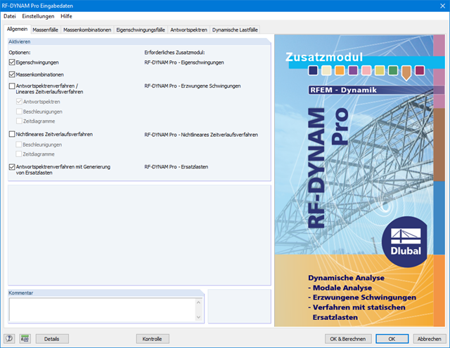
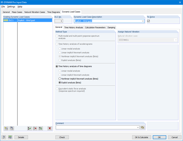
Program proponuje zgodnie z regułami parametry wejściowe odpowiednie dla wybranych norm. Ponadto istnieje możliwość ręcznego wprowadzenia spektrów odpowiedzi. Przypadki obciążeń dynamicznych definiują kierunek efektów spektrum odpowiedzi i wartości własnych konstrukcji, które są istotne dla analizy.
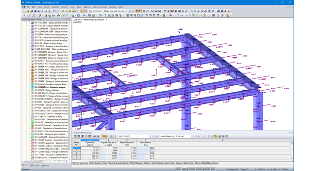
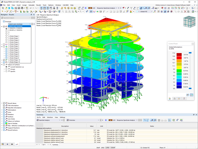
Dzięki integracji RF-/DYNAM Pro z RFEM/RSTAB, można uwzględnić numeryczne i graficzne wyniki z RF-/DYNAM Pro - Forced Vibrations w globalnym raporcie. Ponadto wszystkie opcje programu RFEM umożliwiają wizualizację graficzną.
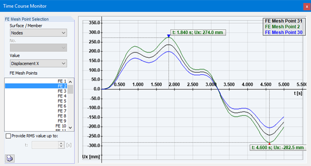
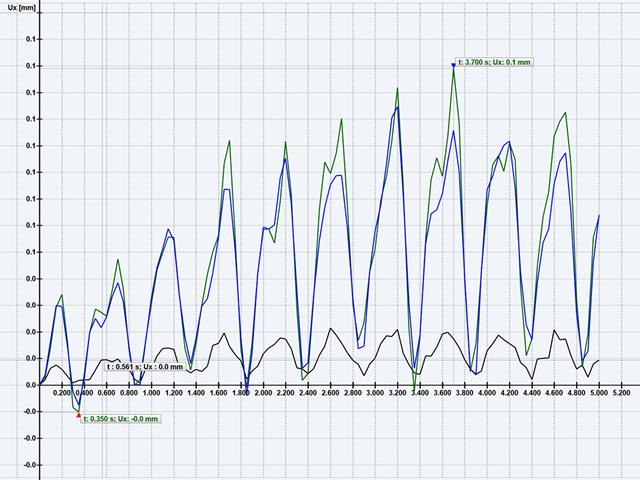
Wyniki analizy przebiegu czasowego są wyświetlane na monitorze przebiegu czasowego. Wszystkie wyniki są wyświetlane w funkcji czasu. Wartości numeryczne można eksportować do aplikacji MS Excel.
W przypadku analizy przebiegu czasowego można wyeksportować wyniki poszczególnych kroków czasowych lub odfiltrować najbardziej niekorzystne wyniki wszystkich kroków czasowych.
Analiza spektrum odpowiedzi generuje kombinacje wyników. Wewnętrznie składowe składowe modalne i składowe kierunkowe oddziaływań sejsmicznych są łączone.
Analiza historii czasowej rozwiązywana jest za pomocą analizy modalnej lub metodą Newmarka. W tym module dodatkowym analiza przebiegu czasowego jest ograniczona do układów liniowych. Chociaż modalna analiza jest szybkim algorytmem, pewna liczba wartości własnych musi być stosowana w celu zapewnienia wymaganej dokładności wyników.
Metoda Newmarka jest bardzo precyzyjną metodą, niezależną od zastosowanej liczby wartości własnych, ale w obliczeniach wymaga odpowiednich niewielkich kroków czasowych. Dla analizy spektrum odpowiedzi równoważne obciążenie statyczne obliczane jest wewnętrznie. Następnie z tej analizy wykonywana jest liniowa analiza statyczna.
Konieczne jest wprowadzenie wymaganych spektrów odpowiedzi, przyspieszeń lub wykresów czasowych. Przypadki obciążeń dynamicznych definiują położenie i kierunek efektów spektrum odpowiedzi, a także czas przyspieszenia lub wzbudzenia siła-czas.
Wykresy czasowe są połączone z przypadkami obciążeń statycznych, co zapewnia dużą elastyczność. W przypadku analizy przebiegu czasowego można zaimportować początkowe odkształcenie z dowolnego przypadku obciążenia lub kombinacji obciążeń.
- Połączenie zdefiniowanych przez użytkownika wykresów czasowych z przypadkami obciążeń lub kombinacjami obciążeń (obciążenia węzłowe, prętowe i powierzchniowe oraz obciążenia wolne i wygenerowane, mogą być łączone z funkcjami o zmiennej czasowej)
- Możliwość połączenia kilku niezależnych funkcji wzbudzenia
- Obszerna biblioteka rejestrów trzęsień ziemi (akcelogramy)
- Analiza przebiegu czasowego rozwiązywana jest za pomocą analizy modalnej lub metodą Newmarka
- Tłumienie konstrukcji przy użyciu współczynnika Rayleigha lub tłumienia Lehra's
- Bezpośredni import początkowych deformacji z przypadków obciążeń lub ich kombinacji
- Graficzne przedstawienie rezultatów na diagramie przebiegu czasowego
- Eksport wyników w zdefiniownych przez użytkownika krokach czasowych lub jako obwiednia
Równoważne obciążenia statyczne generowane są oddzielnie dla każdej miarodajnej postaci drgań własnych oraz kierunku wzbudzenia. Obciążenia są eksportowane do statycznych przypadków obciążeń, a liniowa analiza statyczna wykonywana jest w programie RFEM/RSTAB.

- Spektrum odpowiedzi z wielu norm (ASCE 7-16, NBC 2015 itd.)
- Spektrum odpowiedzi zdefiniowane przez użytkownika lub wygenerowane z akcelerogramów
- Możliwość zadania kierunkowego spektrum odpowiedzi
- Ręczne lub automatyczne wybieranie postaci drgań własnych do analizy spektrum odpowiedzi (można zastosować regułę 5% z EC 8)
- Kombinacje wyników z zastosowaniem superpozycji modalnej (reguła SRSS lub CQC) i superpozycji kierunkowej (reguła SRSS lub 100%/30%)
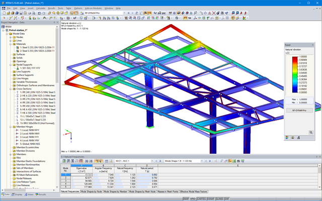
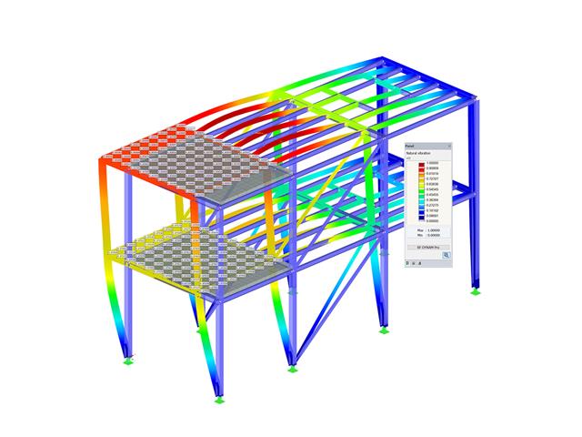
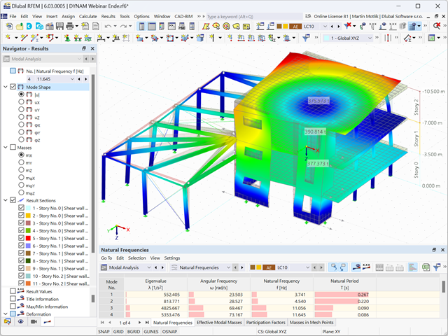
Po zakończeniu obliczeń wyświetlane są postacie drgań własnych, częstotliwości i okresy drgań własnych. Okna z tymi wynikami zintegrowane są z programem głównym RFEM/RSTAB. Postacie drgań własnych konstrukcji zestawione są w tabelach i mogą być wyświetlane graficznie lub jako animacja.
Wszystkie tabele wyników i grafiki stanowią część raportu programu RFEM/RSTAB. Zapewnia to przejrzystą dokumentację obliczeń. Dodatkowo istnieje możliwość eksportu tabel do programu MS Excel.
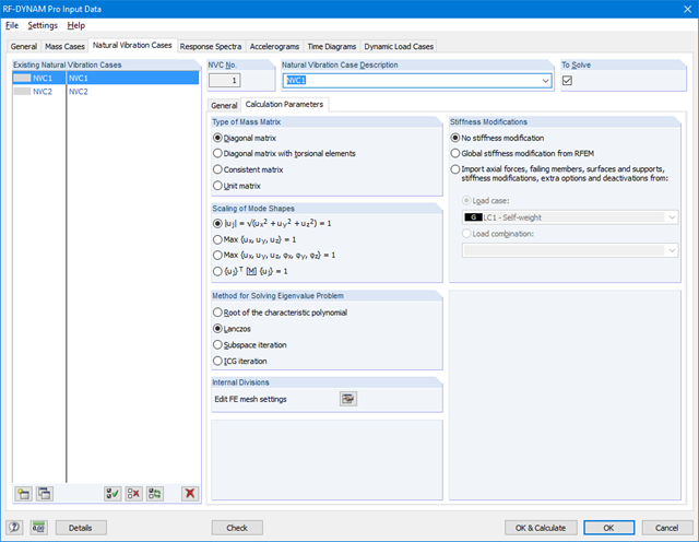
Moduł RF-DYNAM Pro - Natural Vibrations programu RFEM oferuje cztery wydajne solwery wartości własnych:*Pierwiastek wielomianu charakterystycznego
- Metoda Lanchosa
- iteracja podprzestrzeni
- ICG metoda iteracji
W module DYNAM Pro - Natural Vibrations dla RSTAB dostępne są dwie wydajne metody rozwiązywania równań:
- iteracja podprzestrzeni
- Metoda Powera z przesuniętą odwrotnością
Wybór solwera wartości własnych zależy przede wszystkim od rozmiaru modelu.
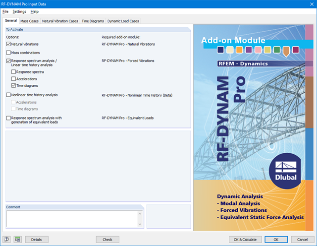
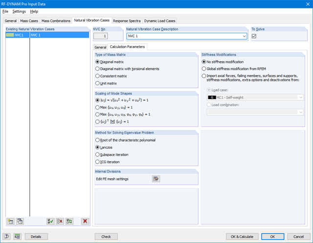
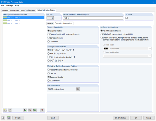
W oknie wprowadzania danych wymagane są wszystkie dane niezbędne do określenia częstotliwości drgań własnych, takie jak kształty masy i solwery wartości własnych.
Moduł dodatkowy RF-/DYNAM Pro-Natural Vibrations określa najniższe wartości własne konstrukcji. Liczbę wartości własnych można dostosować. Masy są importowane bezpośrednio z przypadków obciążeń lub kombinacji obciążeń (z opcjonalnym uwzględnieniem mas całkowitych lub składowej obciążenia w kierunku siły ciężkości).
Dodatkowe masy można zdefiniować ręcznie w węzłach, liniach, prętach lub powierzchniach. Ponadto można kontrolować macierz sztywności poprzez import sił normalnych lub modyfikacji sztywności z przypadku obciążenia lub kombinacji.
- Automatyczne uwzględnianie masy własnej od ciężaru konstrukcji
- Możliwy bezpośredni import mas z przypadków obciążeń lub kombinacji
- Możliwość definicji dodatkowych mas (węzłowych i prętowych mas oraz mas bezwładności)
- Połączenie mas w różnych przypadkach i kombinacjach
- Ustawienie współczynników kombinacji według Eurokodu 8
- Możliwość importowania rozkładu sił (na przykład od stężenia)
- Modyfikacja sztywności (na przykład można importować sztywności nieaktywnych prętów z modułu CONCRETE)
- Możliwe rozważenie utraty podparcia dla niektórych prętów
- Możliwość definiowania kilku przypadków drgań własnych (na przykład w celu analizy różnych mas lub modyfikacji sztywności)
- Wyniki w postaci wartości własnych, częstości kątowych, częstotliwości drgań własnych i okresu drgań własnych
- Określanie postaci drgań i mas w węzłach siatki MES
- Wyniki dla mas modalnych, skutecznych mas modalnych i modalnych współczynników masowych
- Wizualizacja i animacja postaci drgań własnych
- Różne opcje skalowania postaci drgań własnych
- Dokumentacja wyników liczbowych oraz graficznych w protokole wydruku
- Widma odpowiedzi zgodnie z różnymi normami
- Wprowadzono następujące normy:
-
 EN 1998-1:2010 + A1:2013 (Unia Europejska)
 -
 DIN 4149:1981-04 (Niemcy)
 -
DIN 4149:2005-04 (Niemcy)
-
 IBC 2000 (USA)
 -
IBC 2009-ASCE/SEI 7-05 (USA)
-
IBC 2012/15 - ASCE/SEI 7-10 (USA)
-
IBC 2018 - ASCE/SEI 7-16 (USA)
-
 ÖNORM B 4015:2007-02 (Austria)
 -
 NTC 2018 (Włochy)
 -
 NCSE-02 (Hiszpania)
 -
 SIA 261/1:2003 (Szwajcaria)
 -
SIA 261/1:2014 (Szwajcaria)
-
SIA 261/1:2020 (Szwajcaria)
-
 O.G. 23089 + OG 23390 (Turcja)
 -
 SANS 10160-4 2010 (Republika Południowej Afryki)
 -
 SBC 301:2007 (Arabia Saudyjska)
 -
 GB 50011-2001 (Chiny)
 -
GB 50011 - 2010 (Chiny)
-
 NBC 2015 (Kanada)
 -
 DTR BC 2-48 (Algieria)
 -
DTR RPA99 (Algieria)
-
 CFE Sismo 08 (Meksyk)
 -
 CIRSOC 103 (Argentyna)
 -
 NSR - 10 (Kolumbia)
 -
 IS 1893:2002 (Indie)
 -
 AS1170.4 (Australia)
 -
 NCh 433 1996 (Chile)
-
- Dostępne są następujące załączniki krajowe do EN 1998-1:
-
DIN EN 1998-1/NA:2011-01 (Niemcy)
-
ÖNORM EN 1991-1-1:2011-09 (Austria)
-
 NBN-ENV 1998-1-1: 2002 NAD-E/N/F (Belgia)
 -
 ČSN EN 1998-1/NA:2007 (Republika Czeska)
 -
 NF EN 1998-1-1/NA: 2014-09 (Francja)
 -
UNI-EN 1991-1-1/NA:2007 (Włochy)
-
 NP EN 1998-1/NA:2009 (Portugalia)
 -
 SR EN 1998-1/NA:2004 (Rumunia)
 -
 STN EN 1998-1/NA:2008 (Słowacja)
 -
 SIST EN 1998-1: 2005/A101:2006 (Słowenia)
 -
 CYS EN 1998-1/NA:2004 (Cypr)
 -
 NA do BS EN 1998-1:2004:2008 (Wielka Brytania)
 - NS-EN 1998-1:2004 + A1:2013/NA:2014 (Norwegia)
-
- Spektrum odpowiedzi zdefiniowane przez użytkownika
- Możliwość zadania kierunkowego spektrum odpowiedzi
- Odpowiednie kształty drgań dla spektrum odpowiedzi można wybrać ręcznie lub automatycznie (można zastosować regułę 5% z EC 8)
- Wygenerowane równoważne obciążenia statyczne są eksportowane do osobnych przypadków obciążeń dla każdego kierunku oraz przypadku drgań własnych
- Kombinacje wyników według superpozycji modalnej (reguła SRSS i CQC) i superpozycji kierunków (reguła SRSS lub 100%/30%)
- Wyniki z zachowanym znakiem oparte na dominującej postaci drgań własnych mogą być wyświetlane
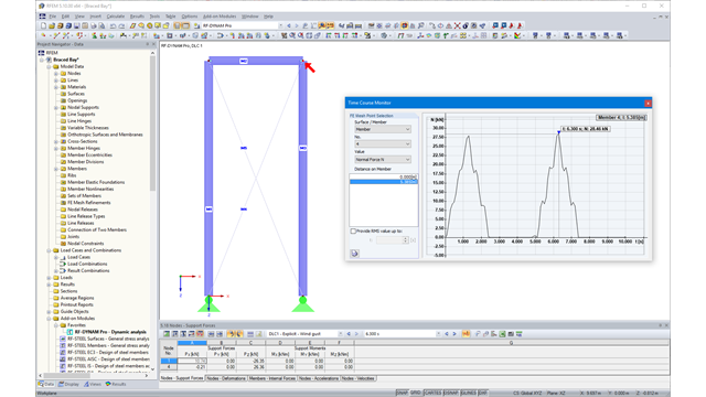
Dzięki integracji RF-/DYNAM Pro z programem RFEM lub RSTAB, do globalnego raportu można włączać numeryczne i graficzne wyniki z RF-/DYNAM Pro - Nonlinear Time History. Ponadto wszystkie opcje w programach RFEM i RSTAB są dostępne do wizualizacji graficznej. Wyniki analizy przebiegu czasowego wyświetlane są na wykresie przebiegu czasowego.
Wyniki są wyświetlane w funkcji czasu, a wartości liczbowe można eksportować do programu MS Excel. Kombinacje wyników mogą być eksportowane jako wynik pojedynczego kroku czasowego lub najbardziej niekorzystne wyniki wszystkich kroków czasowych są odfiltrowywane.
Obliczenia w RFEM
Nieliniowa analiza przebiegu czasowego jest przeprowadzana za pomocą pośredniej analizy Newmarka lub analizy bezpośredniej. Obie metody są metodami bezpośredniej integracji czasu. Analiza pośrednia wymaga definiowania małych kroków czasowych w celu dostarczenia dokładnych wyników. Analiza bezpośrednia określa automatycznie wymagany krok czasowy, w celu zapewnienia stabilności rozwiązania. Analizę bezpośrednią stosuje się w przypadku obliczania krótkotrwałych wzbudzeń, takich jak wzbudzenia impulsowe lub wybuch.
Obliczenia w RSTAB
Nieliniowa analiza przebiegu czasowego jest przeprowadzana z wykorzystaniem analizy bezpośredniej. Jest to metoda bezpośredniej integracji czasu i określa automatycznie krok czasowy, konieczny w celu zapewnienia stabilności wyników obliczeń.

- 001351
- Moduły dodatkowe
- RF-Dynam Pro (en) | Nieliniowa historia czasowa 5
- Analiza dynamiczna i sejsmiczna
RF-/DYNAM Pro - Nonlinear Time History jest zintegrowany z RF‑/DYNAM Pro - Forced Vibrations i rozszerzony o dwie metody analizy nieliniowej (jedna analiza nieliniowa w RSTAB).
Wykresy siła-czas mogą być wprowadzane jako przejściowe, okresowe lub jako funkcje czasu. Dynamiczne przypadki obciążeń stanowią połączenie wykresów czasowych ze statycznymi przypadkami obciążeń, co zapewnia dużą elastyczność. Ponadto, istnieje możliwość definiowania kroków czasowych do obliczeń, tłumienia konstrukcji i opcji eksportu w dynamicznych przypadkach obciążeń.
- 001349
- Ogólne informacje
- RF-Dynam Pro (en) | Nieliniowa historia czasowa 5
- Analiza dynamiczna i sejsmiczna
- Nieliniowe typy prętów, takie jak pręty ściskane i rozciągane lub kable
- Nieliniowości pręta, takie jak uszkodzenie, przerwanie, uplastycznienie pod wpływem rozciągania lub ściskania
- Nieliniowości podpory, takie jak uszkodzenie, tarcie, wykres i częściowa aktywność
- Nieliniowości zwolnienia, takie jak tarcie, częściowa aktywność, wykres oraz uszkodzenie w przypadku, gdy siły wewnętrzne są dodatnie lub ujemne
.png?mw=640&hash=8cfd0c4bd093c03de543d147ffbf6f5c9250634a)
- 001348
- Ogólne informacje
- RF-Dynam Pro (en) | Nieliniowa historia czasowa 5
- Analiza dynamiczna i sejsmiczna
- Zdefiniowane przez użytkownika wykresy czasowe w funkcji czasu, w formie tabelarycznej lub jako obciążenia harmoniczne
- Połączenie wykresów czasowych z przypadkami lub kombinacjami obciążeń w programie RFEM/RSTAB (definiowanie obciążeń węzłowych, prętowych i powierzchniowych oraz zmiennych w czasie obciążeń wolnych i obciążeń)
- Możliwość połączenia kilku niezależnych oddziaływań wzbudzonych
- Nieliniowa analiza przebiegu czasowego z niejawną analizą Newmarka (tylko w RFEM) lub analizą bezpośrednią
- Tłumienie konstrukcji przy użyciu współczynnika Rayleigha lub tłumienia Lehra's
- Bezpośredni import początkowych deformacji z przypadku obciążenia lub kombinacji obciążeń (tylko RFEM)
- Modyfikacje sztywności jako warunki początkowe; na przykład wpływ siły osiowej, dezaktywowane pręty (tylko RSTAB)
- Graficzne przedstawienie rezultatów na diagramie przebiegu czasowego
- Eksport wyników w zdefiniownych przez użytkownika krokach czasowych lub jako obwiednia
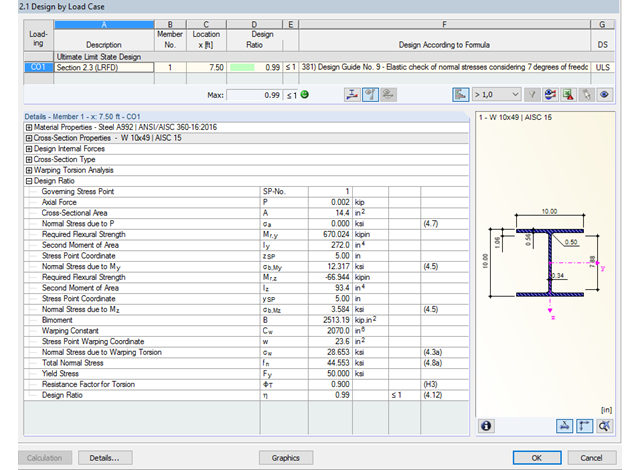
Dzięki zintegrowanemu rozszerzeniu modułu RF-/STEEL Warping Torsion, możliwe jest przeprowadzenie obliczeń zgodnie z Design Guide 9 w RF-/STEEL AISC.
Obliczenia są przeprowadzane z 7 stopniami swobody zgodnie z teorią skręcania skrępowanego i umożliwiają realistyczne obliczenia stateczności z uwzględnieniem skręcania.
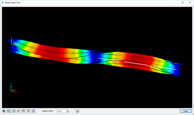
Definiowanie krytycznego momentu wyboczeniowego odbywa się w module RF-/STEEL AISC za pomocą solwera wartości własnych, który umożliwia dokładne określenie krytycznego obciążenia wyboczeniowego.
Solwer wartości własnych pokazuje okno z grafiką wartości własnych, które umożliwia sprawdzenie warunków brzegowych.
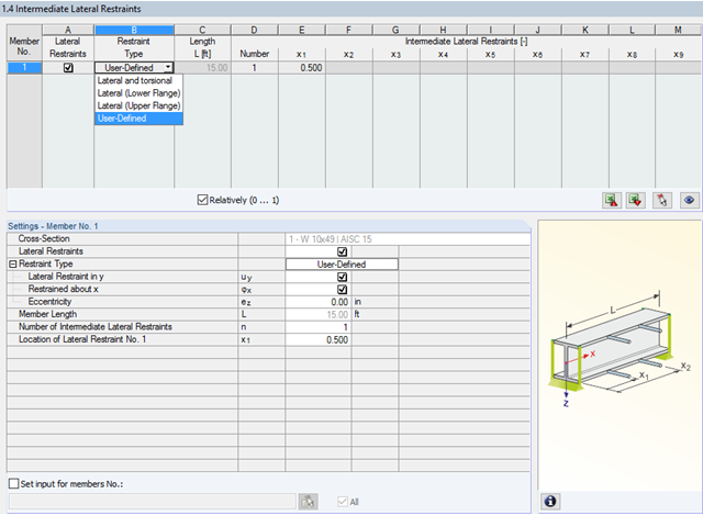
W programie STEEL AISC możliwe jest uwzględnienie pośrednich podpór bocznych w dowolnym miejscu. Na przykład, możliwa jest stabilizacja tylko górnej półki.
Ponadto można przypisać boczne podpory pośrednie zdefiniowane przez użytkownika; na przykład pojedyncze sprężyny obrotowe i sprężyny translacyjne w dowolnym miejscu przekroju.
- Automatyczne uwzględnianie masy własnej od ciężaru konstrukcji
- Możliwy bezpośredni import mas z przypadków obciążeń lub kombinacji
- Opcjonalne definiowanie mas dodatkowych (masy węzłowe, liniowe lub powierzchniowe oraz masy wynikające z bezwładności) bezpośrednio w przypadkach obciążeń
- Opcjonalne pominięcie mas (na przykład masy fundamentów)
- Kombinacje mas w różnych przypadkach i kombinacjach obciążeń
- Predefiniowane współczynniki kombinacji wg różnych norm (EC 8, SIA 261, ASCE 7, ...)
- Opcjonalny import stanów początkowych (np. w celu uwzględnienia naprężenia wstępnego i imperfekcji)
- modyfikacja konstrukcji
- Uwzględnianie uszkodzenia w podporach lub prętach/powierzchniach/bryłach
- Możliwość zadania kilku analiz modalnych (np. w celu analizy różnych mas lub modyfikacji sztywności)
- Wybór typu macierzy mas (macierz diagonalna, macierz spójna, macierz jednostkowa) oraz wskazanych przez użytkownika stopni swobody (translacyjne i rotacyjne)
- Metody określania liczby postaci drgań własnych (liczba zdefiniowana przez użytkownika, liczba określana automatycznie - w celu osiągnięcia zadanych efektywnych współczynników masy modalnej, liczba określana automatycznie - w celu osiągnięcia maksymalnej częstotliwości drgań własnych - dostępne tylko w programie RSTAB)
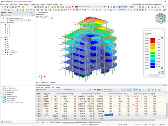
- Określanie postaci drgań i mas w węzłach siatki MES
- Wyniki w postaci wartości własnych, częstości kątowych, częstotliwości drgań własnych i okresu drgań własnych
- Wyniki w postaci mas modalnych, efektywnych mas modalnych, współczynników masy modalnej i współczynników udziału masy
- Tabelaryczne i graficzne przedstawienie mas w punktach siatki MES
- Wizualizacja i animacja postaci drgań własnych
- Różne opcje skalowania postaci drgań własnych
- Dokumentacja wyników numerycznych i graficznych w raporcie
W ustawieniach analizy modalnej należy wprowadzić wszystkie dane, które są niezbędne do określenia częstotliwości drgań własnych. Są to na przykład kształty mas i solwery wartości własnych.
Rozszerzenie Analiza modalna określa najniższe wartości częstości drgań własnych konstrukcji. Liczbę wartości własnych można dostosować lub określić automatycznie. Należy zatem osiągnąć efektywne współczynniki masy modalnej lub maksymalne częstotliwości drgań własnych. Masy są importowane bezpośrednio z przypadków obciążeń i kombinacji obciążeń. W takim przypadku istnieje możliwość uwzględnienia masy całkowitej, składowych obciążenia w globalnym kierunku Z lub tylko składowej obciążenia w kierunku siły ciężkości.
Dodatkowe masy w węzłach, liniach, prętach lub powierzchniach można zdefiniować ręcznie. Ponadto można wpływać na macierz sztywności poprzez import sił osiowych lub modyfikacji sztywności z przypadku obciążenia lub kombinacji obciążeń.
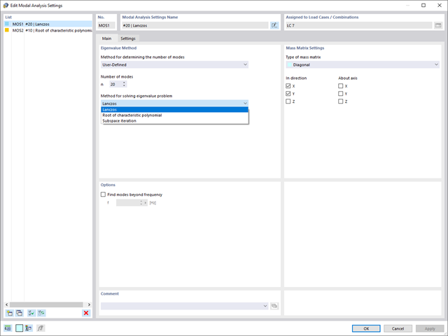
W programie RFEM dostępne są trzy wydajne solwery wartości własnych:
- pierwiastek wielomianu charakterystycznego
- Metoda Lanchosa
- iteracja podprzestrzeni
Z kolei program RSTAB oferuje dwa solwery wartości własnych:
- iteracja podprzestrzeni
- Metoda Powera z przesuniętą odwrotnością
Wybór solwera wartości własnych zależy przede wszystkim od rozmiaru modelu.
Zaraz po zakończeniu obliczeń wyświetlane są wartości własne, częstotliwości drgań własnych i okresy. Okna z tymi wynikami zintegrowane są z programem głównym RFEM/RSTAB. W tabelach można znaleźć wszystkie kształty drgań konstrukcji, a także można je wyświetlić graficznie i animować.
Wszystkie tabele wyników i grafiki stanowią część raportu programu RFEM/RSTAB. Zapewnia to przejrzystą dokumentację obliczeń. Tabele można również eksportować do programu MS Excel.
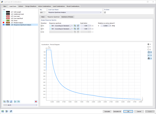
Oprogramowanie do analizy statyczno-wytrzymałościowej firmy Dlubal wykonuje wiele pracy za Ciebie. Program sugeruje zgodnie z regułami parametry wejściowe, istotne dla wybranych norm. Ponadto można ręcznie wprowadzić spektra odpowiedzi.
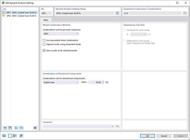
Przypadki obciążeń typu Analiza spektrum odpowiedzi określają kierunek, w którym działają spektra odpowiedzi oraz które wartości własne konstrukcji są istotne dla analizy. W ustawieniach analizy spektralnej można zdefiniować szczegóły dotyczące reguł kombinacji, tłumienia (jeśli ma zastosowanie) i przyspieszenia okresu zerowego (ZPA).
Czy wiecie, że...? Równoważne obciążenia statyczne generowane są oddzielnie dla każdej miarodajnej postaci drgań własnych oraz kierunku wzbudzenia. Obciążenia te są zapisywane w przypadku obciążenia typu Analiza spektrum odpowiedzi, a program RFEM/RSTAB przeprowadza liniową analizę statyczną.
Przypadki obciążeń typu Analiza spektrum odpowiedzi zawierają wygenerowane obciążenia równoważne. Po pierwsze, udziały modalne muszą zostać nałożone na siebie z regułą SRSS lub CQC. W takim przypadku można wykorzystać wyniki podpisane na podstawie dominującego kształtu drgań.
Następnie składowe kierunkowe oddziaływań sejsmicznych są łączone z regułą SRSS lub regułą 100%/30%.
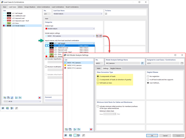
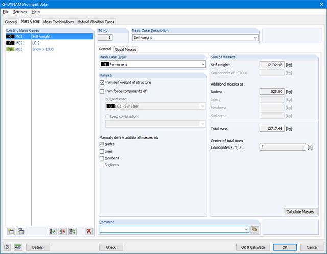
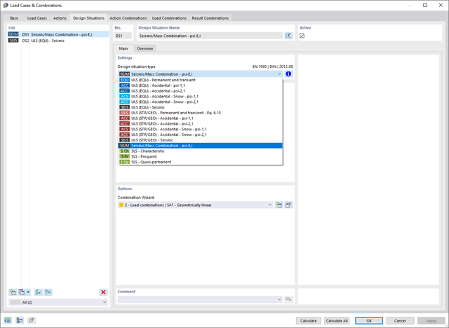
Dostępnych jest kilka opcji definiowania mas dla analizy modalnej. Masy od ciężaru własnego są uwzględniane automatycznie, natomiast obciążenia i masy można uwzględnić bezpośrednio w przypadku obciążenia typu analiza modalna. Potrzebujesz więcej opcji? Należy wybrać, czy obciążenia pełne mają być uwzględniane jako masy, składowe obciążenia w globalnym kierunku Z, czy tylko składowe obciążenia w kierunku siły ciężkości.
Program oferuje dodatkową lub alternatywną opcję importu mas: Ręczna definicja kombinacji obciążeń, począwszy od których masy są uwzględniane w analizie modalnej. Wybrałeś normę obliczeniową? Następnie można utworzyć sytuację obliczeniową typu Kombinacja mas sejsmicznych. W ten sposób program automatycznie oblicza sytuację masową dla analizy modalnej zgodnie z preferowaną normą obliczeniową. Innymi słowy: Program tworzy kombinację obciążeń na podstawie współczynników kombinacji wstępnie ustawionych dla wybranej normy. Zawiera on masy użyte do analizy modalnej.
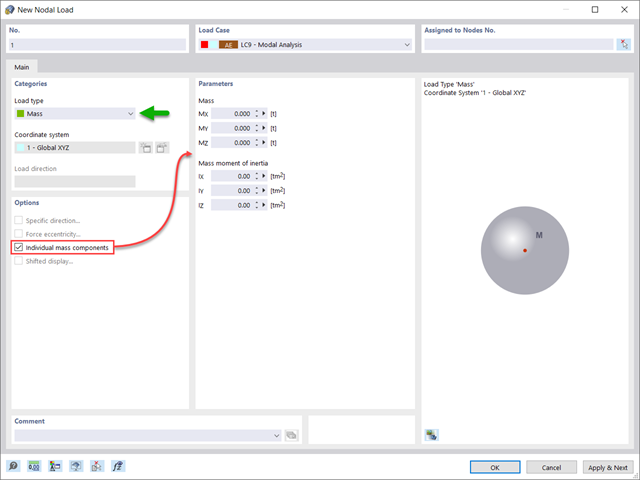
Czy oprócz obciążeń statycznych chcesz uwzględnić również inne obciążenia jako masy? Program umożliwia to dla obciążeń węzłowych, prętowych, liniowych i powierzchniowych. W tym celu podczas definiowania obciążenia należy wybrać typ Obciążenie masą. Dla takich obciążeń należy zdefiniować masę lub składowe masy w kierunkach X, Y i Z. W przypadku mas węzłowych można dodatkowo zdefiniować momenty bezwładności X, Y i Z w celu modelowania bardziej złożonych punktów mas.