32 Results
View Results:
Sort by:
Creating a validation example for Computational Fluid Dynamics (CFD) is a critical step in ensuring the accuracy and reliability of simulation results. This process involves comparing the outcomes of CFD simulations with experimental or analytical data from real-world scenarios. The objective is to establish that the CFD model can faithfully replicate the physical phenomena it is intended to simulate. This guide outlines the essential steps in developing a validation example for CFD simulation, from selecting a suitable physical scenario to analyzing and comparing the results. By meticulously following these steps, engineers and researchers can enhance the credibility of their CFD models, paving the way for their effective application in diverse fields such as aerodynamics, aerospace, and environmental studies.
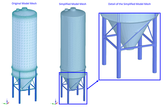
CFD calculations are in general very complex. An accurate calculation of wind flow around complicated structures is very demanding on time and computational costs. In many civil engineering applications, high accuracy is not needed and our CFD program RWIND 2 enables in such cases to simplify the model of a structure and reduce the costs significantly. In this article, some questions about the simplification are answered.
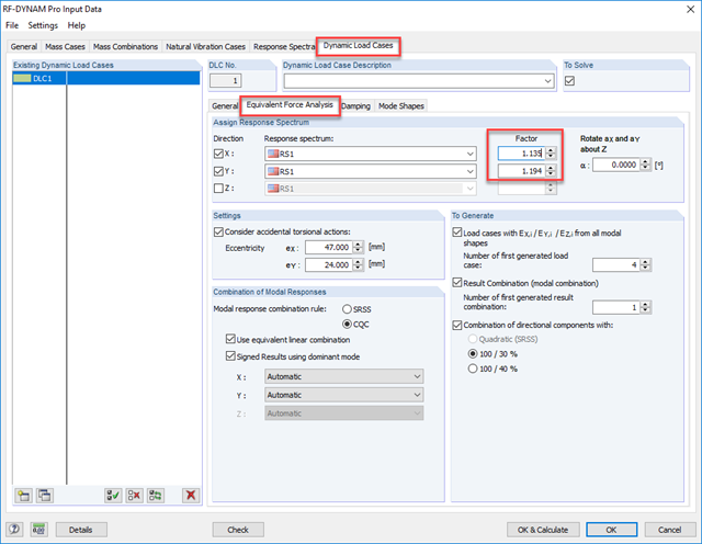
The response spectrum analysis is one of the most frequently used design methods in the case of earthquakes. This method has many advantages. The most important is the simplification: It simplifies the complexity of earthquakes so far that the design can be performed with reasonable effort. The disadvantage of this method is that a lot of information is lost due to this simplification. One way to moderate this disadvantage is to use the equivalent linear combination when combining the modal responses. This article explains this option by describing an example.
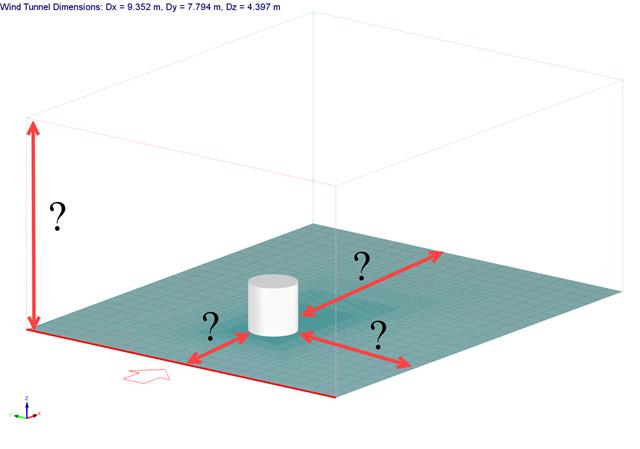
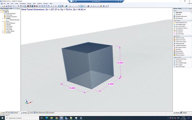
The size of the computational domain (wind tunnel size) is an important aspect of wind simulation that has a significant impact on the accuracy as well as the cost of CFD simulations.
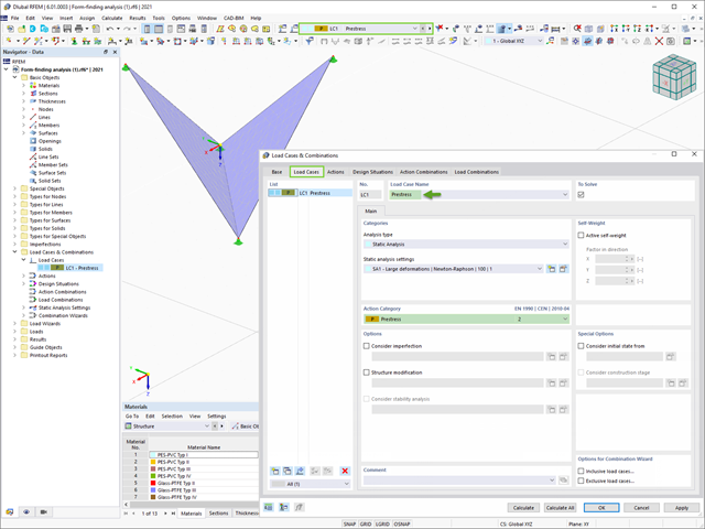
RFEM 6 includes the Form-Finding add-on to determine the equilibrium shapes of surface models subjected to tension and members subjected to axial forces. Activate this add-on in the model's Base Data and use it to find the geometric position in which the prestress of lightweight structures is in equilibrium with the existing boundary conditions.
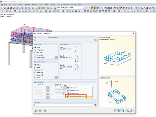
In RFEM and RSTAB, you can generate loads from multilayer composition.
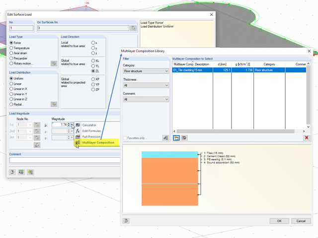
The additional loads from self‑weight are usually composed of several layers; for example, classic floor and ceiling layers in buildings, or road coatings for bridge constructions. When defining load definitions in RFEM and RSTAB, you can use the multi-layer load to define the individual layers with thickness and specific weight.
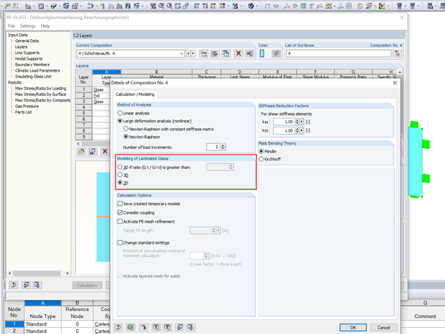
For designing glass in the RF‑GLASS add‑on module, you can use one of two calculation methods: a 2D or a 3D calculation. The main difference between these design options is the automatic modeling of the layers in a temporary model. In a 2D calculation, each layer is generated as a surface element (plate theory); in a 3D calculation, it is generated as a solid. Depending on the selected layer composition, you can either select an option or find it preselected by the program.
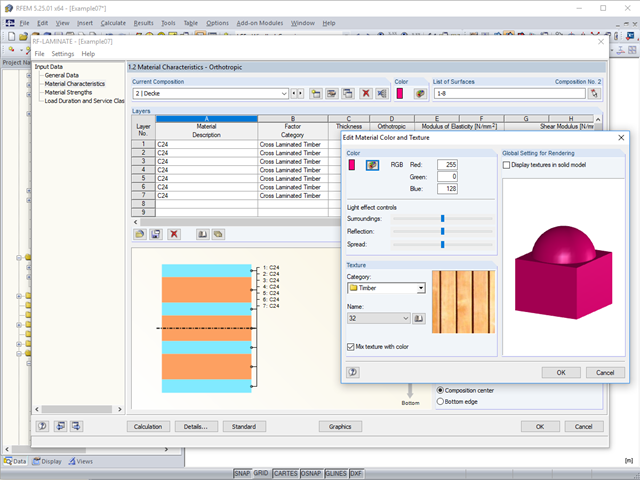
To better distinguish between the different layer compositions (for example, for walls and ceilings), you can assign user‑defined colors and textures to each composition.
The selected increment of the load positions automatically increases the generated load combinations.
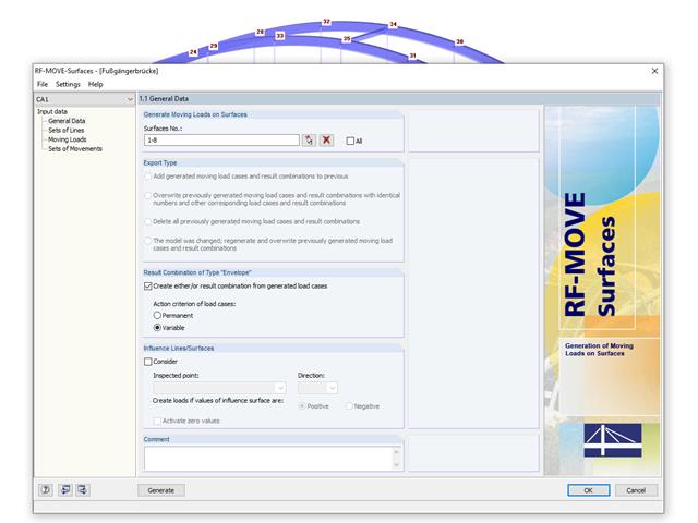
RF-MOVE Surfaces facilitates the generation of load cases from different positions of moving loads. Based on the load positions of the moving load, the program generates separate load cases for RFEM 5. Optionally, an enveloping result combination of all load positions is created.
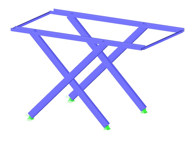
It is necessary to design some structures in different configurations. It may be that an aerial work platform must be analyzed in its position on the ground as well as in the middle and in the extended position. Since such tasks require the creation of several models, which are almost identical, updating all the models with just one mouse click is a considerable relief.
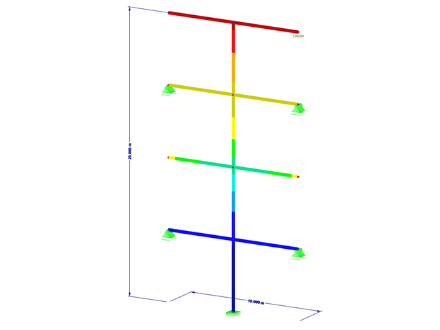
The response spectrum analysis is one of the most frequently used design methods in the case of earthquakes. This method has many advantages. The most important is the simplification: It simplifies the complexity of an earthquake to such an extent that an analysis can be carried out with reasonable effort. The disadvantage of this method is that a lot of information is lost due to this simplification. One way to mitigate this disadvantage is to use the equivalent linear combination when combining the modal responses. This article explains this option by describing an example.
In RFEM and RSTAB, you can use many interfaces to simplify the modeling of your structure. From background layers, to the import of IFC objects that can be converted into members or surfaces, to the import of the entire structural system from Revit or Tekla. Regardless of the performance of the selected interface, further utilization also depends on the accuracy of the imported data.
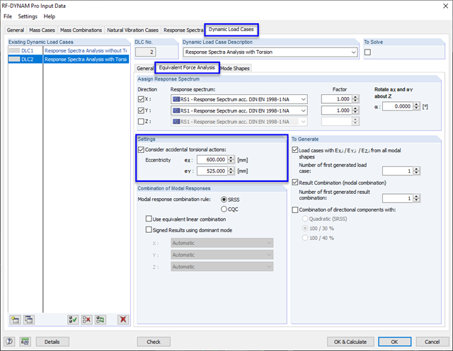
In order to consider inaccuracies regarding the position of masses in a response spectrum analysis, standards for seismic design specify rules that have to be applied in both the simplified and multi-modal response spectrum analyses. These rules describe the following general procedure: The story mass must be shifted by a certain eccentricity, which results in a torsional moment.
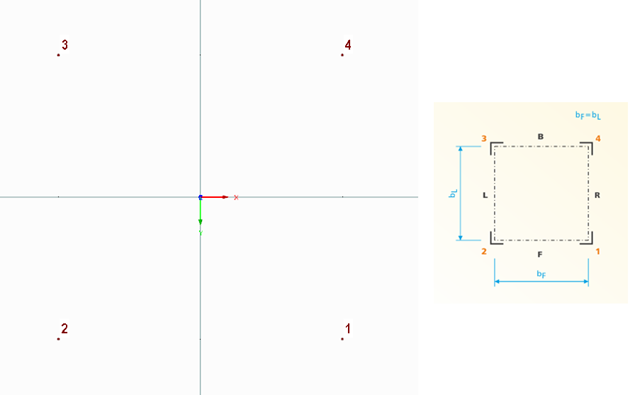
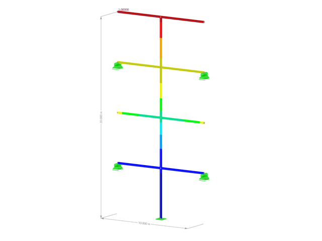
The following technical article describes the creation of a user-defined platform for use on a four-sided tower in the RF-/TOWER add-on modules. First, start with an empty model of the 3D type and define four nodes. The numbering and position of these nodes are very important here.
As gravity loads act on a structure, lateral displacement occurs. In turn, a secondary overturning moment is generated as the gravity load continues to act on the elements in the laterally displaced position. This effect is also known as "P-Delta (Δ)". Sec. 12.9.1.6 of the ASCE 7-16 Standard and the NBC 2015 Commentary specify when P-Delta effects should be considered during a modal response spectrum analysis.
In the case of a post-critical failure, a substantial change occurs in the geometry of a structure. After reaching the instability of the equilibrium, a stable, strength position is reached again. The post-critical analysis requires an experimental approach. It is necessary to manually load the structure in increments, step by step.
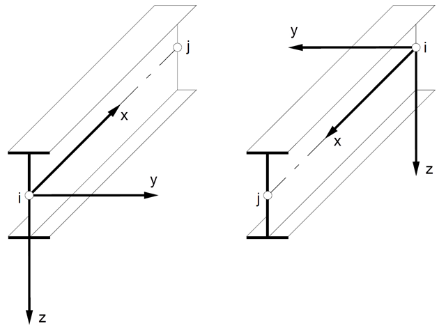
In spatial structures, the member position plays an important role in terms of determining internal forces. The orientation of member axes can be defined either by a global cross-section rotation angle, or by a specific member rotation angle. These two angles are added to determine the position of the main axes of a member in a 3D model.
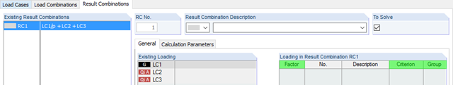
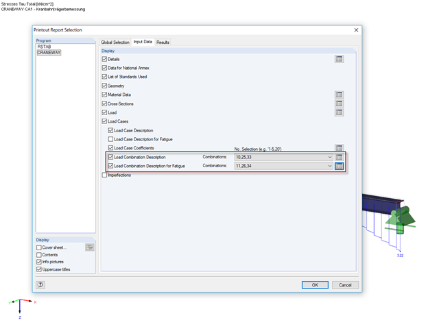
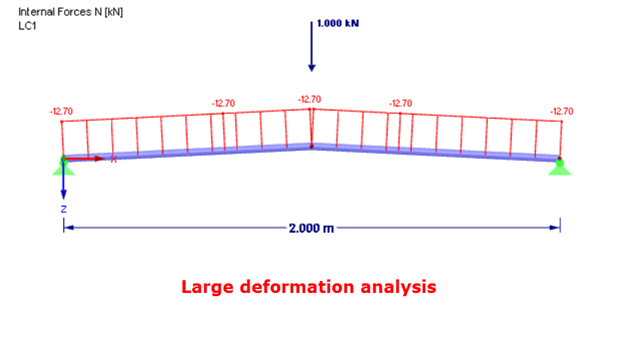
RFEM and RSTAB provides two different methods for the superposition of load cases. Using load combinations, the loads of individual load cases are superimposed and calculated in a "big load case". On the other hand, result combinations only combine the results of the individual load cases. This article describes the with the basis of defining result combinations and explain it in detail on two examples.
Nodal supports are usually defined with regard to the global axis system. However, it is sometimes necessary to rotate the nodal support. For example, for a floor slab with a pile foundation. For geological reasons, the piles do not rest in the ground vertically, but in an inclined position. Each end point of the piles has a nodal support that can only absorb forces along the pile foundation direction. Therefore, rotating the nodal support is required. Various options for this are described in previous posts.
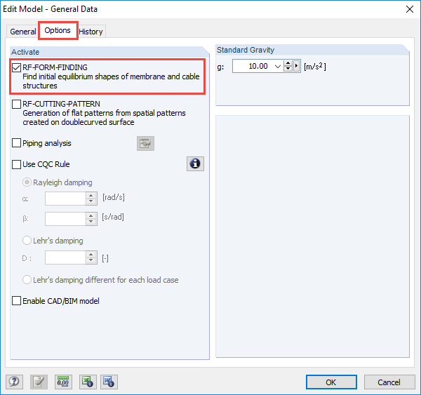
The RF-FORM-FINDING add-on module determines equilibrium shapes of membrane and cable elements in RFEM. In this calculation process, the program searches for such geometric position where the surface stress/prestress of membranes and cables is in equilibrium with natural and geometric boundary conditions. This process is called form-finding (hereinafter referred to as FF). The FF calculation can be activated in RFEM globally in the "General Data" of a model, "Options" tab. After selecting the corresponding option, a new load case or a calculation process called RF-FORM-FINDING is created in RFEM. An additional FF parameter is available for defining surface stress and prestress when entering cables and membranes. By activating the FF option, the program always starts the form-finding process before the pure structural calculation of internal forces, deformation, eigenvalues, etc., and generates a corresponding prestressed model for further analysis.
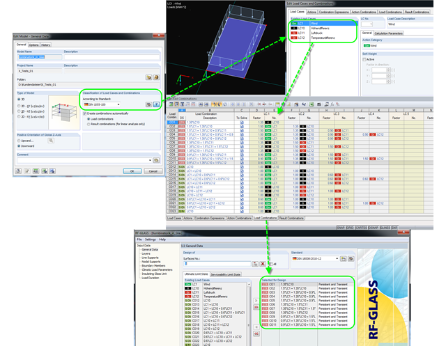
For the superposition or combination of loads, the German standard DIN 18008 refers to DIN 1055‑100. This also applies for the individual parameters of climatic loads to be transferred. In this case, it is possible to summarize the temperature change and meteorological pressure change in a single load and to define the local altitude change as a permanent load.
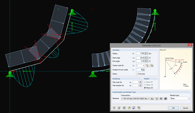
In addition to straight beams, it is sometimes necessary to calculate or design arched or circular beams in RSTAB. For this purpose, there is a special feature under "Tools" → "Generate Model – Members" → "Circle". You can easily use this tool to generate a full or pitch circle. The most important parameter here is the number of new nodes, which affects the accuracy of the results.
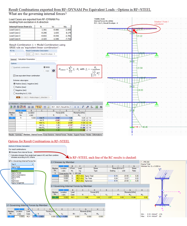
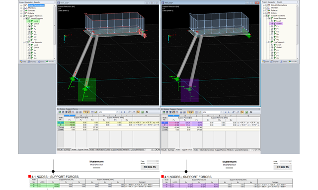
Result combinations exported from RF‑/DYNAM Pro – Equivalent Loads are generated by superimposing the results from the individual modal responses. For this, the SRSS rule can be used as "equivalent linear combination". When result combinations are used in RF‑/STEEL, two options are available for calculating stresses. In the first option, the results from the result combinations are used directly. This is done line by line, for each maximum and minimum controlling internal force. In the second option, stresses are determined from the individual load cases. The quadratic superposition rule is then performed again in RF-/STEEL.
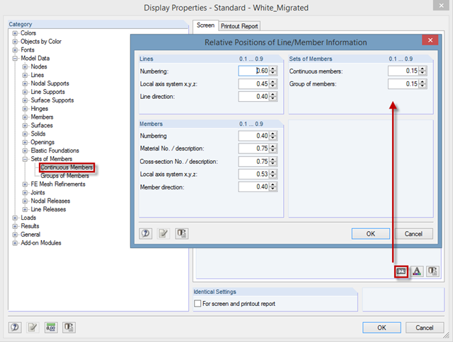
In RFEM and RSTAB, you can arrange the labeling of lines, members, and sets of members in a user‑defined way. To do this, open the dialog box in "Display Properties", where you can define the position of the information about the relative distance from the member start.
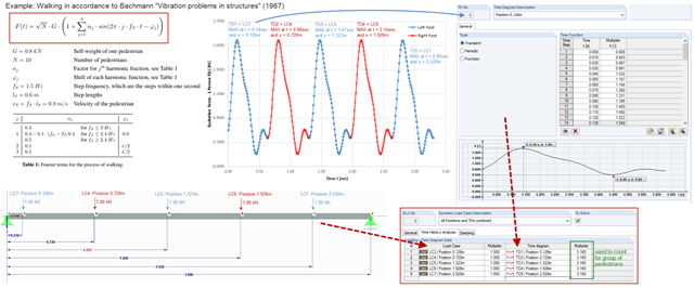
To simulate an excitation that varies over time and changes its position, you can combine several loading time diagrams in RF‑/DYNAM Pro - Forced Vibrations.
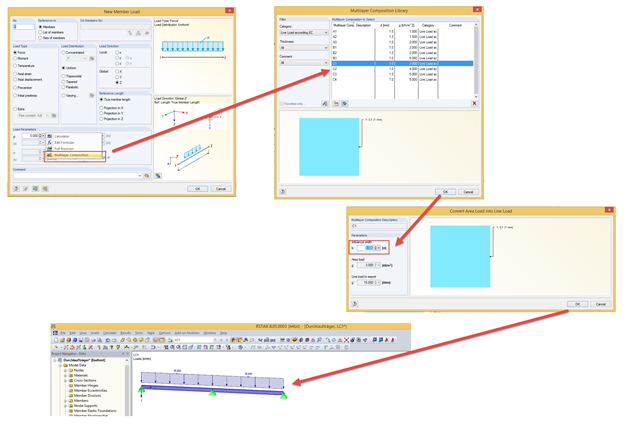
In addition to manually entering values, you can enter line loads in the "Member Load" dialog box using the "Multi-Layer Composition" function. This is a library that contains the compositions of several layers for applying loads. You can freely specify the layer structure using the parameters of description, thickness, density, or surface load, and comment for each layer.
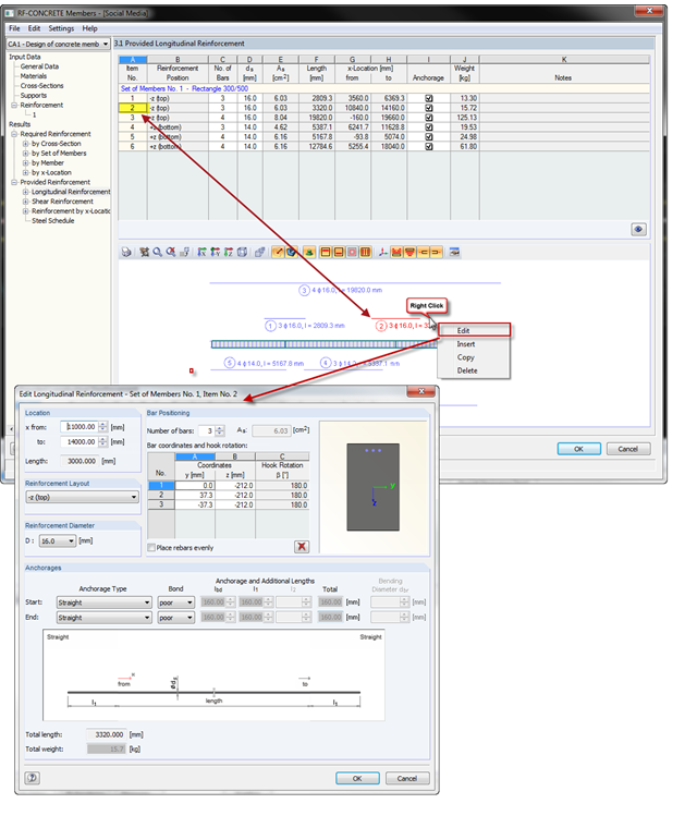
With the introduction of OSG graphics for the representation of design reinforcement in RF‑CONCRETE Members and CONCRETE, you can also select the reinforcement position directly in the graphic. Right-click the mouse to open the context menu where you can edit, copy, or delete the selected reinforcement position.
RF-LAMINATE allows free definition of materials. Thus, you can combine any compositions of different materials. The combination of concrete and timber is possible as well. However, the rigid composite must be provided when defining such a composition. In RF-LAMINATE, you can consider full shear coupling or no shear coupling at all.