50 Wyniki
Wyświetl wyniki:
Sortuj według:
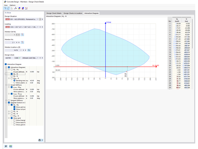
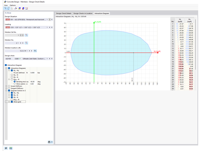
Czy wiesz, że wykresy interakcji moment-siła (wykresy MN) można wyświetlić również graficznie? Umożliwia to wyświetlenie nośności przekroju w przypadku interakcji momentu zginającego i siły osiowej. Oprócz wykresów interakcji związanych z osiami przekroju (wykres My-N i wykres Mz-N) można również wygenerować indywidualny wektor momentów w celu utworzenia wykresu interakcji Mres -N. Płaszczyznę przekroju wykresów MN można wyświetlić na wykresie interakcji 3D.Program wyświetla odpowiednie pary wartości stanu granicznego nośności w tabeli. Tabela jest dynamicznie powiązana z wykresem, dzięki czemu wybrany punkt graniczny jest również wyświetlany na wykresie.
- 002469
- Ogólne informacje
- Projektowanie konstrukcji betonowych RFEM 6
- Projektowanie konstrukcji betonowych RSTAB 9
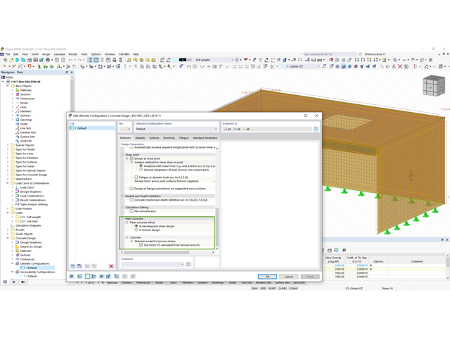
Pracujesz z elementami konstrukcyjnymi składającymi się z płyt? W takim przypadku należy przeprowadzić obliczenia na ścinanie z uwzględnieniem wymagań obliczania przebicia, na przykład zgodnie z 6.4, EN 1992-1-1. Oprócz płyt stropowych można w ten sposób wymiarować również płyty fundamentowe.
W konfiguracji stanu granicznego nośności dla wymiarowania betonu można zdefiniować parametry obliczeń przebicia dla wybranych węzłów.
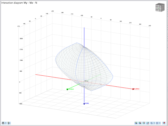
Projektowanie konstrukcji betonowych | Wykres interakcji My-Mz-N (3D) przekrojów z betonu zbrojonego
Na pytanie 'Ile można przewozić?' zazwyczaj odpowiada 'Tak'. Do graficznego przedstawiania stanu granicznego nośności przekrojów żelbetowych wymagany jest trójwymiarowy wykres interakcji momentu-momentu-siła osiowa. Oprogramowanie do analizy statyczno-wytrzymałościowej firmy Dlubal właśnie to oferuje.
Dzięki dodatkowemu wyświetleniu oddziaływania obciążenia można łatwo rozpoznać lub zwizualizować przekroczenie granicznej nośności przekroju żelbetowego. Ponieważ możesz kontrolować właściwości wykresu, możesz dostosować wygląd wykresu My-Mz-N do swoich potrzeb.
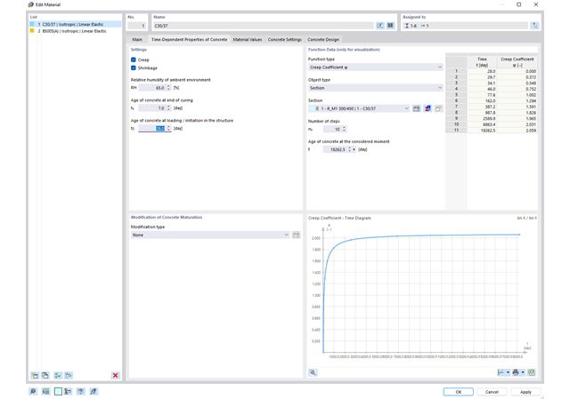
Właściwości betonu, zależne od czasu, takie jak pełzanie i skurcz, są bardzo ważne dla obliczeń. Można je zdefiniować bezpośrednio dla materiału w programie do analizy statyczno-wytrzymałościowej. W oknie dialogowym do wprowadzania danych wyświetlany jest przebieg czasowy funkcji pełzania lub skurczu. Można łatwo wybrać modyfikację zastosowanego wieku betonu, na przykład ze względu na obróbkę termiczną.
.png?mw=640&hash=5a991f211d984ac624978f514e70c53da263e5d9)
W zależności od siły osiowej N, można wygenerować linię krzywizny momentu dla dowolnego wektora momentu. Program pokazuje również pary wartości wyświetlanego wykresu w tabeli. Ponadto można aktywować jako dodatkowy wykres sieczny i sztywność styczną przekroju żelbetowego, należące do wykresu krzywizny momentu.
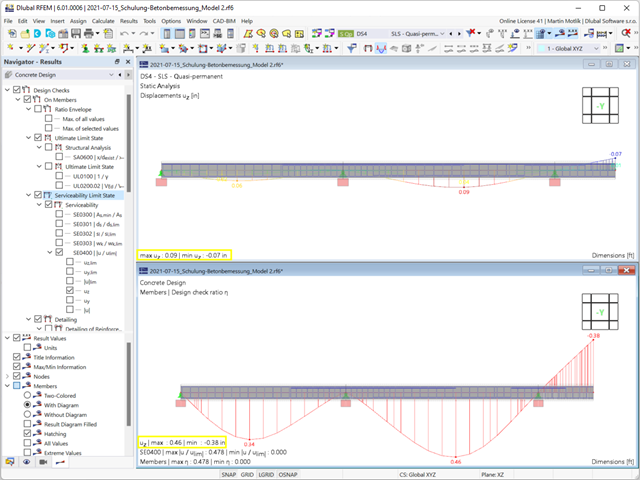
Odkształcenie prętów i powierzchni jest określane z uwzględnieniem zarysowanego (stan II) lub niezarysowanego (stan I) przekroju żelbetowego. Podczas określania sztywności można uwzględnić usztywnienie przy rozciąganiu między rysami, zwane 'usztywnieniem przy rozciąganiu', zgodnie z zastosowaną normą obliczeniową.
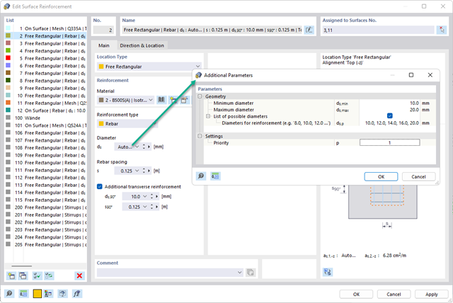
Istniejące zbrojenie powierzchniowe można automatycznie zaprojektować tak, aby pokryć wymagane zbrojenie. Można wybrać, czy automatycznie ma być definiowana średnica zbrojenia, czy też rozstaw prętów.
Przejdź do filmu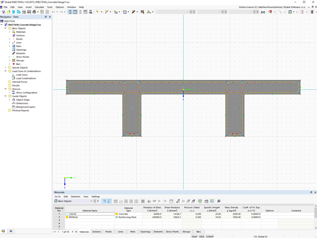
W rozszerzeniu Projektowanie konstrukcji betonowych można wymiarować dowolny przekrój RSECTION. Otulinę betonową, zbrojenie na ścinanie i zbrojenie podłużne definiuje się bezpośrednio w RSECTION.
Po zaimportowaniu przekroju ze zbrojeniem RSECTION do programu RFEM 6, można go również wykorzystać do obliczeń w rozszerzeniu Projektowanie konstrukcji betonowych.
Przejdź do filmu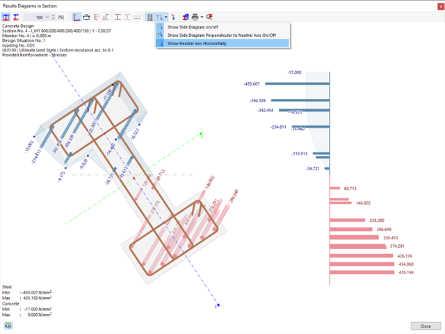
Istniejące naprężenia i odkształcenia przekroju betonowego i zbrojenia można wyświetlić w postaci obrazu naprężeń 3D lub grafiki 2D. W zależności od tego, które wyniki zostaną wybrane w drzewie wyników, naprężenia lub odkształcenia są wyświetlane w zdefiniowanym zbrojeniu podłużnym pod oddziaływaniami obciążeń lub granicznymi siłami wewnętrznymi.
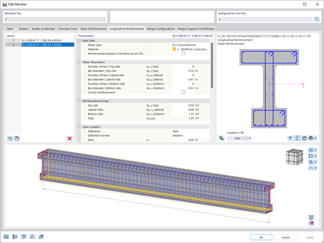
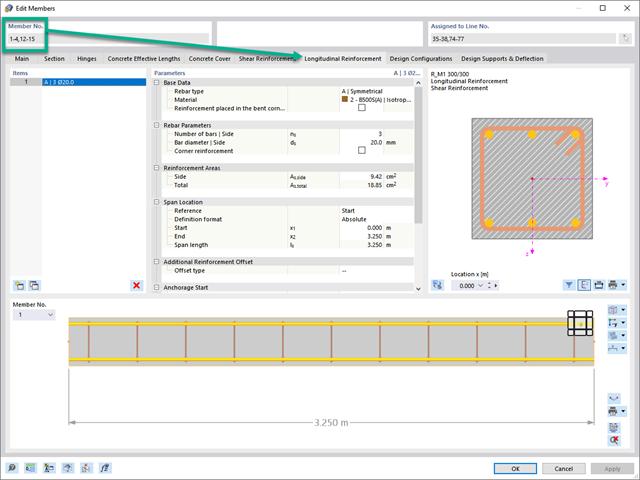
Zbrojenie na ścinanie i zbrojenie podłużne można zdefiniować indywidualnie dla każdego pręta. W tym przypadku dostępne są różne szablony do wprowadzania zbrojenia.
Czy chcesz określić nośność przekroju żelbetowego na zginanie dwukierunkowe? W tym celu należy najpierw aktywować wykres interakcji moment-moment (wykres My-Mz). Wykres My-Mz przedstawia poziomy przekrój przez trójwymiarowy wykres dla określonej siły osiowej N. Dzięki połączeniu z trójwymiarowym wykresem interakcji można tam również zwizualizować płaszczyznę przekroju.
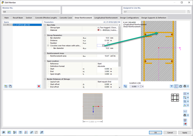
W zakładce "Zbrojenie na ścinanie" można wybrać opcję "Powiązania krzyżowe na wolnych prętach zbrojeniowych z aktywnym wyborem w oknie graficznym". Pozwala to na umieszczenie dodatkowych powiązań krzyżowych na wolnych prętach zbrojenia podłużnego.
Pozycję więzów krzyżowych można aktywować lub dezaktywować w infografice. Powiązania krzyżowe są uwzględniane podczas kontroli stanu granicznego nośności i obliczeń konstrukcji. Są one dostępne dla obliczeń zgodnie z EN 1992-1-1.
Przejdź do filmu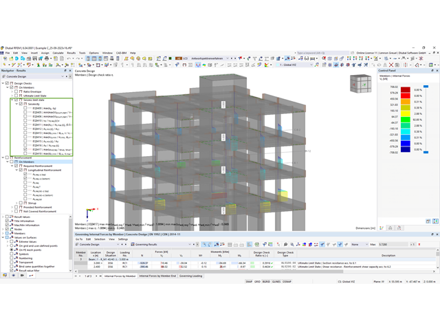
W rozszerzeniu Projektowanie konstrukcji betonowych można przeprowadzać obliczenia sejsmiczne dla prętów żelbetowych zgodnie z EC 8. Są to między innymi następujące funkcje:
- Konfiguracje obliczeń sejsmicznych
- Rozróżnianie klas ciągliwości DCL, DCM, DCH
- Możliwość przeniesienia współczynnika odpowiedzi z analizy dynamicznej
- Sprawdzenie wartości granicznej współczynnika odpowiedzi
- Weryfikacja nośności dla "Wytrzymały słup - słaba belka"
- Uszczegółowienie i reguły szczególne dla współczynnika ciągliwości krzywizny
- Uszczegółowienie i reguły szczególne dla ciągliwości lokalnej
Teraz w rozszerzeniu Projektowanie konstrukcji betonowych można wymiarować elementy wykonane z betonu zbrojonego włóknami zgodnie z wytyczną "DAfStb Steel Fiber-Reinforced Concrete".
Ta opcja jest dostępna dla obliczeń zgodnie z EN 1992-1-1. Obliczenia zgodnie z wytyczną DAfStb są przeprowadzane po przypisaniu betonu typu "Fibrobeton" do elementu konstrukcyjnego z betonu zbrojonego.
Przejdź do filmu.png?mw=640&hash=3c928fddb4215c3df06e0b731d5c3f2e475cd9db)
W ramach jednego pręta można zdefiniować szerokość integracyjną i efektywną szerokość płyty belek teowych (żeber) o różnych szerokościach. Pręt jest podzielony na segmenty. Przejście między różnymi szerokościami półek można sortować lub określać liniowo. Ponadto program umożliwia uwzględnienie zdefiniowanego zbrojenia powierzchni jako zbrojenia pasa przy wymiarowaniu żebra w betonie zbrojonym.
- 002557
- Ogólne informacje
- Projektowanie konstrukcji betonowych RFEM 6
- Projektowanie konstrukcji betonowych RSTAB 9
Skorzystaj i oszczędzaj czas! Ta funkcja umożliwia jednoczesne definiowanie lub edycję zbrojenia dla kilku prętów lub zbiorów prętów.
Przejdź do filmu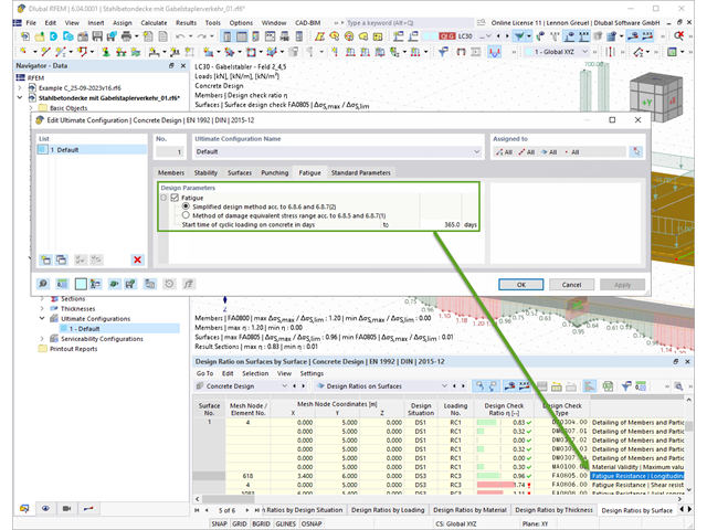
Rozszerzenie Projektowanie konstrukcji betonowych umożliwia wymiarowanie prętów i powierzchni ze względu na zmęczenie zgodnie z EN 1992-1-1, rozdział 6.8.
W przypadku obliczeń zmęczenia można opcjonalnie wybrać dwie metody lub poziomy obliczeniowe w konfiguracjach obliczeniowych:
- Poziom obliczeniowy 1: Obliczenia uproszczone wg. do 6.8.6 i 6.8.7(2) Kryterium uproszczone jest stosowane dla częstych kombinacji oddziaływań zgodnie z EN 1992-1-1, rozdział 6.8.6 (2) oraz EN 1990, równ. (6.15b) wraz z obciążeniami od ruchu drogowego w stanie użytkowalności. Dla stali zbrojeniowej sprawdzany jest maksymalny zakres naprężeń zgodnie z 6.8.6. Naprężenie ściskające w betonie jest określane za pomocą górnego i dolnego dopuszczalnego naprężenia zgodnie z 6.8.7(2).
- Poziom analizy 2: Obliczanie równoważnego naprężenia niszczącego zgodnie z 6.8.5 i 6.8.7(1) (uproszczone obliczenia na zmęczenie): Obliczenia z wykorzystaniem zakresów równoważnych naprężeń niszczących są przeprowadzane dla kombinacji zmęczeniowych, zgodnie z EN 1992-1-1, rozdział 6.8.3, równ. (6.69) o specyficznie zdefiniowanym oddziaływaniu cyklicznym Qfat .
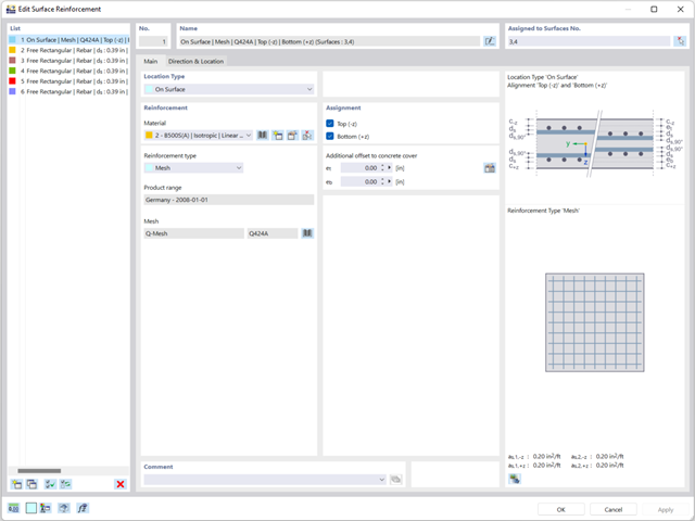
Zbrojenie powierzchniowe należy wprowadzić bezpośrednio na poziomie programu RFEM. W takim przypadku można indywidualnie wybrać zdefiniowane zbrojenie powierzchniowe. Podczas wprowadzania zbrojenia powierzchniowego do dyspozycji użytkownika są standardowe funkcje Kopiuj, Odbij lub Obróć.
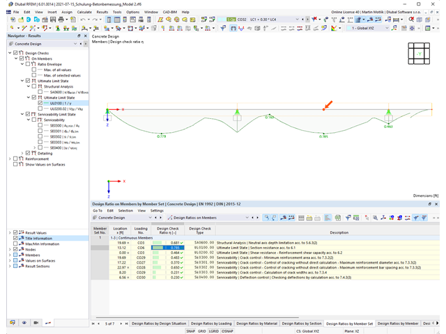
Program do analizy statyczno-wytrzymałościowej zapewnia przejrzysty przegląd wszystkich przeprowadzonych kontroli obliczeń dla określonej normy obliczeniowej. Dla każdego warunku projektowego należy określić kryterium obliczeniowe. Oprócz sprawdzania stanu granicznego nośności i użytkowalności program sprawdza zasady projektowania określone w normie. Dla każdej kontroli obliczeń są określone szczegóły obliczeń, w tym wartości początkowe, wyniki pośrednie i wyniki końcowe. Proces obliczeń wraz z zastosowanymi wzorami, standardowymi źródłami i wynikami szczegółowo przedstawiony jest w oknie informacyjnym w szczegółach obliczeń.
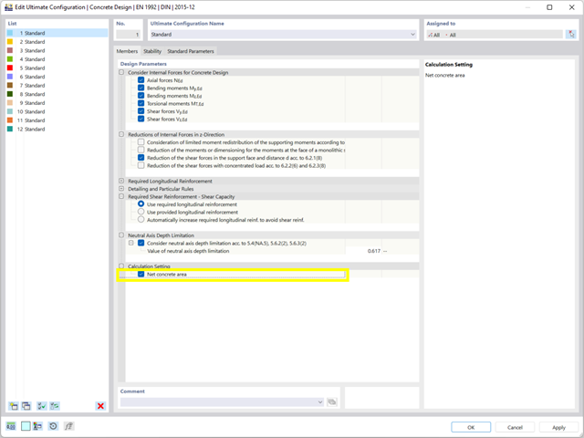
Podczas wymiarowania przekroju można bezpośrednio określić, czy powierzchnia betonowa zostanie zastosowana za prętami zbrojeniowymi, czy też zostanie odjęta od przekroju betonowego. Istnieje możliwość obliczenia przekroju betonu netto, zwłaszcza w przypadku przekroju silnie zbrojonego.
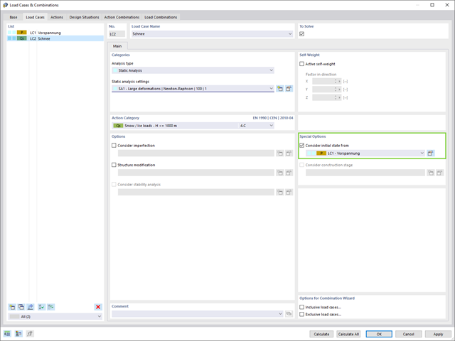
Czy wiesz dokładnie, w jaki sposób przebiega wyszukiwanie kształtu? Po pierwsze, proces znajdowania kształtu przypadków obciążeń z kategorią przypadku obciążenia "Wstępne naprężenie" przesuwa początkową geometrię siatki do optymalnie zrównoważonej pozycji za pomocą iteracyjnych pętli obliczeniowych. W tym celu program wykorzystuje metodę Zaktualizowanej Strategii Odniesienia (URS) opracowaną przez prof. Bletzingera i prof. Ramma. Technologię tę charakteryzują kształty równowagi, które po obliczeniach prawie dokładnie odpowiadają początkowo zadanym warunkom brzegowym (ugięcie, siła i naprężenie wstępne).
Oprócz opisu oczekiwanych sił lub zwisów na elementach, zintegrowane podejście URS umożliwia również uwzględnienie sił regularnych. W całym procesie pozwala to na przykład na opisanie ciężaru własnego lub ciśnienia pneumatycznego za pomocą odpowiednich obciążeń elementów.
Wszystkie te opcje dają rdzeniu obliczeniowemu możliwość obliczania postaci antyklastycznych i synklastycznych, które są w równowadze sił, dla geometrii płaskich lub obrotowo-symetrycznych. Aby możliwe było realistyczne zaimplementowanie obu typów, pojedynczo lub razem w jednym środowisku, w obliczeniach dostępne są dwa sposoby opisania wektorów sił do analizy form-finding:
- Metoda rozciągania - opis znajdowania kształtu wektorów sił w przestrzeni dla geometrii płaskich
- Metoda rzutowania - opis znajdowania kształtu wektorów sił na płaszczyznę rzutowania z ustaleniem położenia poziomego dla geometrii stożkowych
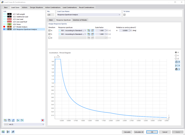
Czy wiecie, że...? Równoważne obciążenia statyczne generowane są oddzielnie dla każdej miarodajnej postaci drgań własnych oraz kierunku wzbudzenia. Obciążenia te są zapisywane w przypadku obciążenia typu Analiza spektrum odpowiedzi, a program RFEM/RSTAB przeprowadza liniową analizę statyczną.

- 002232
- Ogólne informacje
- Optymalizacja i koszty | Szacowanie emisji CO2 RFEM 6
- Optymalizacja i koszty | Szacowanie emisji CO2 RSTAB 9
Możesz być pewien, że koszty są ważnym czynnikiem w planowaniu konstrukcyjnym każdego projektu. Należy również przestrzegać przepisów dotyczących szacowania emisji. Dwuczęściowe rozszerzenie Optymalizacja i koszty/Szacowanie emisji CO2 ułatwia odnalezienie się w gąszczu norm i opcji. Wykorzystuje technologię sztucznej inteligencji (AI) optymalizacji rojem cząstek (PSO) w celu znalezienia odpowiednich parametrów dla sparametryzowanych modeli i bloków, które zagwarantują zgodność ze zwykłymi kryteriami optymalizacji. Ponadto, rozszerzenie oszacowuje koszty modelu lub emisję CO2 poprzez określenie kosztów jednostkowych lub emisji jednostkowej dla materiałów zdefiniowanych w modelu konstrukcyjnym. Dzięki temu rozszerzeniu jesteś po bezpiecznej stronie.
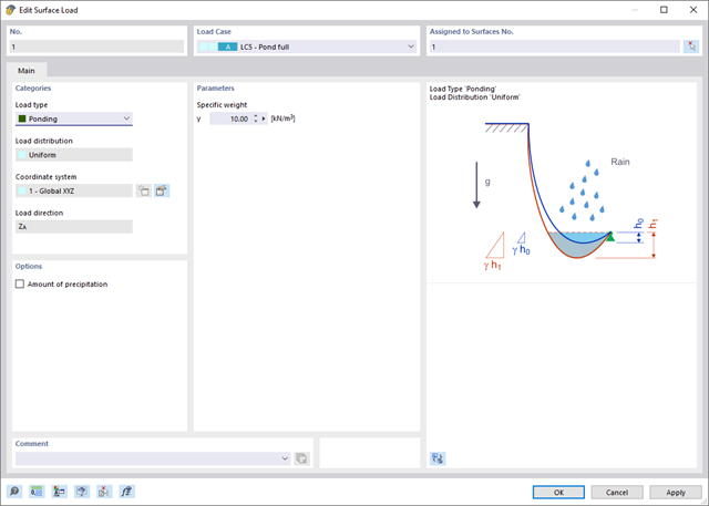
Wprowadzenie typu obciążenia Woda stojąca umożliwia symulację oddziaływań deszczu na powierzchnie wielokrotnie zakrzywione, z uwzględnieniem przemieszczeń według analizy dużych odkształceń.
Ten numeryczny proces analizy deszczowej analizuje przypisaną geometrię powierzchni i określa, które składowe wody deszczowej spływają, a które gromadzą się w postaci kałuży (kieszeni wodnych) na powierzchni. Rozmiar kałuży powoduje wówczas odpowiednie obciążenie pionowe do analizy statyczno-wytrzymałościowej.
Funkcja ta jest przeznaczona do analizy w przybliżeniu poziomych geometrii dachów membranowych pod obciążeniem deszczem.
Przejdź do filmu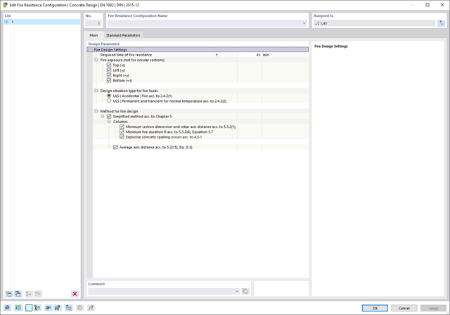
- 002691
- Ogólne informacje
- Projektowanie konstrukcji betonowych RFEM 6
- Projektowanie konstrukcji betonowych RSTAB 9
W rozszerzeniu Projektowanie konstrukcji betonowych można przeprowadzić uproszczone obliczenia odporności ogniowej słupów (Rozdział 5.3.2) i belek (Rozdział 5.6), zgodnie z EN 1992-1-2.
W przypadku uproszczonych obliczeń odporności ogniowej dostępne są następujące metody weryfikacji:
- Słupy: Minimalne wymiary przekroju prostokątnego i okrągłego wg tabeli 5.2a oraz równania 5.7 do obliczania czasu ekspozycji pożarowej
- Belki: Minimalne wymiary i odległości między środkami zgodnie z Tabelą 5.5 i Tabelą 5.6
Siły wewnętrzne do obliczeń odporności ogniowej można wyznaczyć przy użyciu dwóch metod.
- 1: W tym przypadku siły wewnętrzne z wyjątkowej sytuacji obliczeniowej są bezpośrednio uwzględniane w obliczeniach.
- 2: Siły wewnętrzne z obliczeń w temperaturze normalnej są redukowane za pomocą współczynnika Eta,fi (ηfi) i są następnie wykorzystywane do obliczeń odporności ogniowej.
Ponadto istnieje możliwość modyfikacji rozstawu osi zgodnie z równ. 5.5.
W porównaniu z modułem dodatkowym RF-FORM-FINDING (RFEM 5), do modułu Form-Finding dla programu RFEM 6 dodano następujące nowe funkcje:
- Określenie wszystkich warunków brzegowych dotyczących obciążenia dla analizy znajdowania kształtu (form-finding) w pojedynczym przypadku obciążenia
- Przechowywanie wyników analizy znajdowania kształtu jako stanu początkowego z możliwością późniejszego wykorzystania przy dalszej analizie modelu
- Automatyczne przypisywanie stanu początkowego z analizy znajdowania kształtu do wszystkich sytuacji obciążeniowych w sytuacji obliczeniowej za pomocą kreatorów kombinacji
- Dodatkowe geometryczne warunki brzegowe dla prętów (długość elementu nieobciążonego, maksymalny zwis w pionie, zwis w pionie w najniższym punkcie punkcie)
- Dodatkowe warunki brzegowe z uwagi na obciążenie w analizie znajdowania kształtu dla prętów (maksymalna siła w pręcie, minimalna siła w pręcie, rozciągająca składowa pozioma, rozciąganie na i-końcu, rozciąganie na końcu j, minimalne rozciąganie na końcu i, minimalne rozciąganie na końcu j)
- Typ materiału „Tkanina” i „Folia” w bibliotece materiałów
- Równoległe analizy znajdowania kształtu w jednym modelu
- Symulacja kolejnych etapów znajdowania kształtów w połączeniu z rozszerzeniem Analiza etapów konstrukcji (CSA)
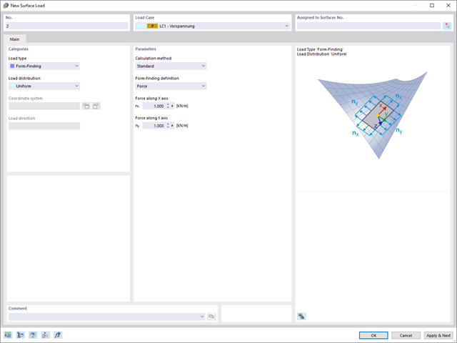
Po aktywowaniu rozszerzenia Form-Finding w Danych ogólnych, efekt znajdowania kształtu jest przypisywany do przypadków obciążeń z kategorią przypadków obciążenia "Sprężenie" w połączeniu z obciążeniami od znajdowania kształtu od pręta, powierzchni i bryły wczytaj katalog. Jest to przypadek obciążenia wstępnego naprężenia. Przekształca się on zatem w analizę znajdowania kształtu dla całego modelu ze zdefiniowanymi w nim wszystkimi elementami prętowymi, powierzchniowymi i bryłowymi. Do znajdowania kształtu odpowiednich elementów prętowych i membranowych dochodzi się w całym modelu za pomocą specjalnych obciążeń w zakresie znajdowania kształtu i regularnych definicji obciążeń. Te obciążenia znajdowania kształtu opisują oczekiwany stan odkształcenia lub siły po wyszukaniu kształtu w elementach. Obciążenia regularne opisują zewnętrzne obciążenie całego układu.
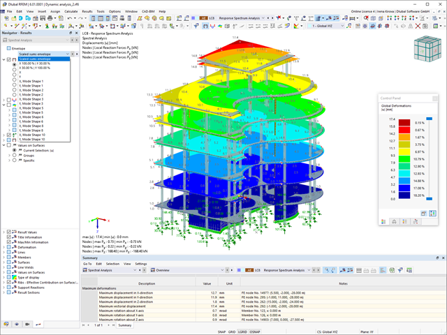
Przypadki obciążeń typu Analiza spektrum odpowiedzi zawierają wygenerowane obciążenia równoważne. Po pierwsze, udziały modalne muszą zostać nałożone na siebie z regułą SRSS lub CQC. W takim przypadku można wykorzystać wyniki podpisane na podstawie dominującego kształtu drgań.
Następnie składowe kierunkowe oddziaływań sejsmicznych są łączone z regułą SRSS lub regułą 100%/30%.
W porównaniu z modułem dodatkowym RF-/DYNAM Pro-Equivalent Loads (RFEM 5/RSTAB 8) do rozszerzenia Analiza spektrum odpowiedzi dla programu RFEM 6/RSTAB 9 dodano następujące nowe funkcje:
- Spektrum odpowiedzi z wielu norm (EN 1998, DIN 4149, IBC 2018 itd.)
- Spektrum odpowiedzi zdefiniowane przez użytkownika lub wygenerowane z akcelerogramów
- Możliwość zadania kierunkowego spektrum odpowiedzi
- Aby zapewnić przejrzystość wyniki są przechowywane łącznie, w jednym przypadku obciążenia, w ramach którego dostępne są różne poziomy wyświetlania
- Wpływ przypadkowych oddziaływań skręcających może być uwzględniany automatycznie
- Automatyczne kombinacje obciążeń sejsmicznych z innymi przypadkami obciążeń, możliwe do wykorzystania w wyjątkowej sytuacji obliczeniowej
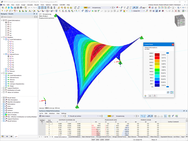
Proces znajdowania kształtu tworzy model konstrukcyjny z aktywnymi siłami w "przypadku obciążenia sprężonego" Ten przypadek obciążenia pokazuje przemieszczenie od początkowego położenia wejściowego do ustalonej geometrii w wynikach deformacji. W wynikach opartych na sile lub naprężeniach (siły wewnętrzne prętów i powierzchni, naprężenia w bryłach, ciśnienia gazu itp.) określany jest stan w celu zachowania znalezionej formy. Do analizy kształtu geometrycznego program oferuje dwuwymiarowy wykres konturowy z przedstawieniem wysokości bezwzględnej i wykresem nachylenia do wizualizacji sytuacji na zboczu.
Teraz przeprowadzane są dalsze obliczenia i analiza statyczno-wytrzymałościowa całego modelu. W tym celu program przenosi geometrię zorientowaną na kształt wraz z odkształceniami zależnymi od elementów do uniwersalnego stanu początkowego. Można go teraz używać w przypadkach obciążeń i kombinacjach obciążeń.