
When generating shear walls and deep beams, you can assign not only surfaces and cells, but also members.

You can neglect openings with a certain area in the building model calculation. This function can be activated in the global settings of the building stories. A warning message appears saying that the openings have been neglected.
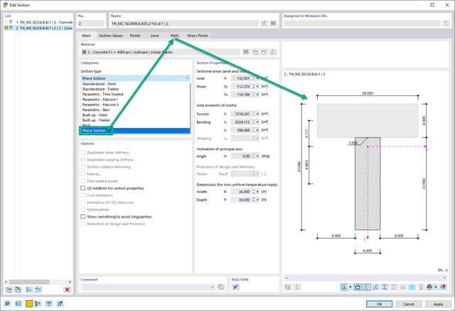
In the Construction Stages Analysis (CSA) add-on, you can use built-up cross-sections by means of what are known as phase sections. This allows you to activate and deactivate the parts of the "Parametric - Massive II" section type throughout the construction stages.

In the Geotechnical Analysis add-on, the Hoek-Brown material model is available. The model shows linear-elastic ideal-plastic material behavior. Its nonlinear strength criterion is the most common failure criterion for stone and rocks.
You can enter the material parameters using
- Rock parameters directly, or alternatively via
- GSI classification.
Detailed information about this material model and the definition of the input in RFEM can be found in the respective chapter Hoek-Brown Model of the online manual for the Geotechnical Analysis add-on.

The building model is calculated in two phases:
- Global 3D calculation of the global model, where the slabs are modeled as a rigid plane (diaphragm) or as a bending plate
- Local 2D calculation of the individual floors
After the calculation, the results of the columns and walls from the 3D calculation and the results of the slabs from the 2D calculation are combined in a single model. This means that there is no need to switch between the 3D model and the individual 2D models of the slabs. The user only works with one model, saves valuable time, and avoids possible errors in the manual data exchange between the 3D model and the individual 2D ceiling models.
The vertical surfaces in the model can be divided into shear walls and opening lintels. The program automatically generates internal result members from these wall objects, so they can be designed as members according to any standard in the Concrete Design add-on.
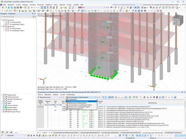
Shear walls and deep beams of a building model are available as independent objects in the design add-ons. This allows for faster filtering of the objects in results, as well as better documentation in the printout report.
The building story generator in the Building Model add-on allows you to automatically create building stories, depending on the topology of the model.

For a response spectrum analysis of building models, you can display the sensitivity coefficients for the horizontal directions by story.
These key figures allow you to interpret the sensitivity to stability effects.

The modal relevance factor (MRF) can help you to assess to which extent specific elements participate in a specific mode shape. The calculation is based on the relative elastic deformation energy of each individual member.
The MRF can be used to distinguish between local and global mode shapes. If multiple individual members show significant MRF (for example, > 20%), the instability of the entire structure or a substructure is very likely. On the other hand, if the sum of all MRFs for an eigenmode is around 100%, a local stability phenomenon (for example, buckling of a single bar) can be expected.
Furthermore, the MRF can be used to determine critical loads and equivalent buckling lengths of certain members (for example, for stability design). Mode shapes for which a specific member has small MRF values (for example, < 20%) can be neglected in this context.
The MRF is displayed by mode shape in the result table under Stability Analysis --> Results by Member --> Effective Lengths & Critical Loads.

The Concrete Design add-on allows you to perform the seismic design of reinforced concrete members according to EC 8. This includes, among other things, the following functionalities:
- Seismic design configurations
- Differentiation of the ductility classes DCL, DCM, DCH
- Option to transfer the behavior factor from a dynamic analysis
- Check of the limit value for the behavior factor
- Capacity design checks of "Strong column - weak beam"
- Detailing and particular rules for curvature ductility factor
- Detailing and particular rules for local ductility

Several modeling tools are available for elements in building models:
- Vertical line
- Column
- Wall
- Beam
- Rectangular floor
- Polygonal floor
- Rectangular floor opening
- Polygonal floor opening
This feature allows you to define the element on the ground plane (for example, with a background layer) with the associated multiple element creation in space.

Using the "Load Transfer Only" story type, you can consider slabs without stiffness effect in and out of the plane in the Building Model add-on. This element type collects the loads on the slab and transfers them to the supporting elements of a 3D model. Thus, you can simulate secondary components, such as grillage and similar load distribution elements, without any further effect in the 3D model.

Have you activated the Building Model add-on? Very good! This allows you to display the center of rigidity in tabular and graphical form. Use it for your dynamic analysis, for example.
.png?mw=640&hash=55038d2a1591f62179796666cb9b2fede0274e19)
A graphical and tabular output of the results for deformations, stresses, and strains helps you when determining the soil solids. To achieve this, use the special filter criteria for targeted selection of results.
The program doesn't leave you alone with the results. If you want to graphically evaluate the results in the soil solids, you can use the guide objects. For example, you can define clipping planes. This allows you to view the corresponding results in any plane of the soil solid.
And not just that. The utilization of result sections and clipping boxes facilitates the precise graphical analysis of the soil solid.
You already know that it is possible to model and analyze a soil and a structure in the entire model. As a result, you have explicitly taken into account the soil-structure interaction. By modifying a component, you achieve the immediate correct consideration in the analysis as well as in the results for the entire system of the soil and structure.

Are you ready for the evaluation? Use the calculation diagrams, which show the distribution of a specific result during the calculation.
You can freely define the layout of the vertical and horizontal axes of the calculation diagram. This allows you, for example, to consider the settlement distribution of a certain node, depending on the load.

Your data are always documented in a multilingual printout report. You can adjust the content at any time and save it as a template. You can also add graphics, texts, MathML formulas, and PDF documents to your report with just a few clicks.

Enter and model a soil solid directly in RFEM. You can combine the soil material models with all common RFEM add-ons.
This allows you to easily analyze the entire models with a complete representation of the soil-structure interaction.
All parameters required for the calculation are automatically determined from the material data that you have entered. The program then generates the stress-strain curves for each FE element.

Did you know? You can enter the soil layers that you have obtained from the subsoil expertises done in the locations into the program in the form of soil samples. Assign the explored soil materials, including their material properties, to the layers.
For the definition of the samples, you can enter the data in tables as well as in the respective editing dialog box. Furthermore, you can also specify the groundwater level in the soil samples.

The soil solids that you want to analyze are summarized in soil massifs.
Use the soil samples as a basis for a definition of the respective soil massif. This way, the program allows for user-friendly generation of the massif, including the automatic determination of the layer interfaces from the sample data, as well as the groundwater level and the boundary surface supports.
Soil massifs provide you with the option to specify a target FE mesh size independently of the global setting for the rest of the structure. You can thus consider the various requirements of the building and soil in the entire model.

Do you want to model and analyze the behavior of a soil solid? To ensure this, special suitable material models have been implemented in RFEM.
You can use the modified Mohr-Coulomb model with a linear-elastic ideal-plastic model or a nonlinear elastic model with an oedometric stress-strain relation. The limit criterion, which describes the transition from the elastic area to that of the plastic flow, is defined according to Mohr-Coulomb.

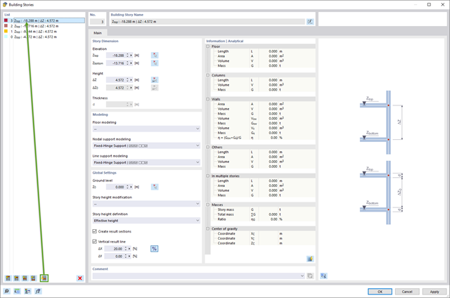
Are you afraid that your project will end in the digital tower of Babel? The Building Model add-on for RFEM supports you in your work on a construction project with several stories. It allows you to define a building by means of stories at specified elevations. You can adjust the stories in many ways afterwards and also select the story slab stiffness. Information about the stories and the entire model (center of gravity, center of rigidity) is displayed for you in tables and graphics.

- 002232
- General
- Optimization & Cost / CO2 Emission Estimation for RFEM 6
- Optimization & Cost / CO2 Emission Estimation for RSTAB 9
You can be sure that costs are an important factor in the structural planning of any project. It is also essential to adhere to the provisions on emissions estimation. The two-part add-on Optimization & Costs/CO2 Emission Estimation makes it easier for you to find your way through the jungle of standards and options. It uses the artificial intelligence technology (AI) of the particle swarm optimization (PSO) to find the right parameters for parameterized models and blocks that guarantee the compliance with the usual optimization criteria. This add-on also estimates the model costs or CO2 emissions by specifying unit costs or emissions per material definition for the structural model. With this add-on, you are on the safe side.

Compared to the RF-/DYNAM Pro - Equivalent Loads add-on module (RFEM 5 / RSTAB 8), the following new features have been added to the Response Spectrum Analysis add-on for RFEM 6 / RSTAB 9:
- Response spectra of numerous standards (EN 1998, DIN 4149, IBC 2018, and so on)
- User-defined response spectra or those generated from accelerograms
- Direction-relative response spectrum approach
- Results are stored centrally in a load case with underlying levels to ensure clarity
- Accidental torsional actions can be taken into account automatically
- Automatic combinations of seismic loads with the other load cases for use in an accidental design situation

Compared to the RF‑SOILIN add-on module (RFEM‑5), the following new features have been added to the Geotechnical Analysis add-on for RFEM 6:
- Creation of the layered soil as a 3D model from the entirety of the defined soil samples
- Recognized material law according to Mohr-Coulomb for soil simulation
- Graphical and tabular output of stresses and strains at any depth of the soil
- Optimal consideration of the soil-structure interaction on the basis of an overall model

Compared to the RF‑/STABILITY (RFEM 5) and RSBUCK (RSTAB 8) add-on modules, the following new features have been added to the Structure Stability add-on for RFEM 6 / RSTAB 9:
- Activation as a property of a load case or a load combination
- Automated activation of the stability calculation via combination wizards for several load situations in one step
- Incremental load increase with user-defined termination criteria
- Modification of the mode shape normalization without recalculation
- Result tables with filter option

Compared to the RF‑/STAGES add-on module (RFEM 5), the following new features have been added to the Construction Stages Analysis (CSA) add-on for RFEM 6:
- Consideration of construction stages at RFEM level
- Integration of the construction stage analysis into the combinatorics in RFEM
- Additional structural elements, such as line hinges, are supported
- Analysis of alternative construction processes in a model
- Reactivation of elements

- 002108
- General
- Optimization & Cost / CO2 Emission Estimation for RFEM 6
- Optimization & Cost / CO2 Emission Estimation for RSTAB 9
- Artificial intelligence technology (AI): Particle swarm optimization (PSO)
- Structure optimization according to the minimum weight or deformation
- Use of any number of optimization parameters
- Specification of variable ranges
- Optimization of cross-sections and materials
- Parameter definition types
- Optimization | Ascending or Optimization | Descending
- Application of parametric models and blocks
- Code-based JavaScript parametrization of blocks
- Optimization taking into account the design results
- Tabular display of the best model mutations
- Real-time display of the model mutations in the optimization process
- Model cost estimation by specifying unit prices
- Determination of the global warming potential GWP when realizing the model by estimating the CO2 equivalent
- Specification of weight-, volume-, and area-based units (price and CO2e)

- 002109
- General
- Optimization & Cost / CO2 Emission Estimation for RFEM 6
- Optimization & Cost / CO2 Emission Estimation for RSTAB 9
Did you know? The structural optimization in the programs RFEM and RSTAB is a completion of the parametric input. It is a parallel process beside the actual model calculation with all its regular calculation and design definitions. The add-on assumes that your model or block is built with a parametric context and is controlled in its entirety by global control parameters of the "optimization" type. Therefore, these control parameters have a lower and upper limit and a step size to delimit the optimization range. If you want to find optimal values for the control parameters, you have to specify an optimization criterion (for example, minimum weight) with the selection of an optimization method (for example, particle swarm optimization).
You can already find the cost and CO2 emission estimation in the material definitions. You can activate both options individually in each material definition. The estimation is based on a unit for unit cost or unit emission for members, surfaces, and solids. In this case, you can select whether to specify the units by weight, volume, or area.

- 002110
- General
- Optimization & Cost / CO2 Emission Estimation for RFEM 6
- Optimization & Cost / CO2 Emission Estimation for RSTAB 9
There are two methods that you can use for the optimization process, with which you can find optimal parameter values according to a weight or deformation criterion.
The most efficient method with the littlest calculation time is the near-natural particle swarm optimization (PSO). Have you heard or read about it? This artificial intelligence (AI) technology has a strong analogy to the behavior of flocks of animals, looking for a resting place. In such swarms, you can find many individuals (cf. optimization solution - for example, weight) who like to stay in a group and follow the group movement. Let's assume that each individual swarm member has a need to rest at an optimal resting place (cf. best solution - for example, lowest weight). This need increases as the resting place is approached. Thus, the swarm behavior is also influenced by the properties of the space (cf. result diagram).
Why the excursion into biology? Quite simply – the PSO process in RFEM or RSTAB proceeds in a similar way. The calculation run starts with an optimization result from a random assignment of the parameters to be optimized. It repeatedly determines new optimization results with varied parameter values, which are based on the experience of the previously performed model mutations. The process continues until the specified number of possible model mutations is reached.
As an alternative to this method, the program also offers you a batch processing method. This method attempts to check all possible model mutations by randomly specifying the values for the optimization parameters until a predetermined number of possible model mutations is reached.
After calculating a model mutation, both variants also check the respective activated design results of the add-ons. Furthermore, they save the variant with the corresponding optimization result and value assignment of the optimization parameters if the utilization is < 1.
You can determine the estimated total costs and emission from the respective sums of the individual materials. The sums of the materials are composed of the weight-based, volume-based, and area-based partial sums of the member, surface, and solid elements.