
In RFEM and RSTAB, you can visualize the flow field quantities of pressure, velocity, turbulence kinetic energy, and turbulence dissipation rate for the wind simulation.
The clipping planes are aligned with the respective wind direction.
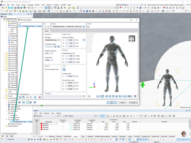
In RFEM 6 and RSTAB 9, you have the option to enter "Visual Objects" as guide objects. You can import the file formats 3ds, stl, and obj.
These objects allow you to create a better reference to the dimensions.
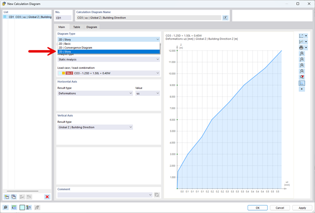
The "2D | Story" calculation diagram type is used to create result diagrams via the building axis. This allows you to easily analyze the behavior of the entire building under static and dynamic effects.
You can use this diagram type, for example, to visualize the seismic force over the building height.
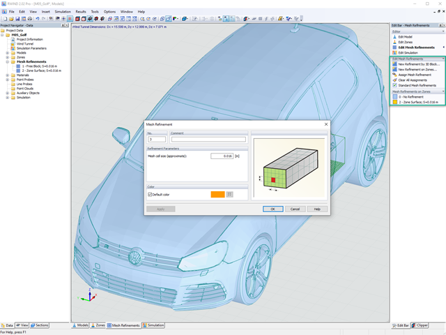
Do you already know the editor for mesh refinement control? It is a great help for your work! Why? It's easy – it gives you the following options:
- Graphic visualization of the areas with mesh refinements
- Mesh refinement of zones
- Deactivating the standard 3D solid mesh refinement with transversion into the corresponding manual 3D mesh refinements.
These options help you to formulate a suitable rule for meshing the entire model, even for the models with unusual dimensions. Use the editor to efficiently define small model details on large buildings or detailed meshing areas in the coating area of the model. You will be amazed!

As you've already learned, the results of a Modal Analysis load case are displayed in the program after a successful calculation. You can thus immediately see the first mode shape graphically or as an animation. You can also easily adjust the representation of the mode shape standardization. Do that directly in the Results navigator, where you have one of four options for the visualization of the mode shapes available for the selection:
- Scaling the value of the mode shape vector uj to 1 (considers the translation components only)
- Selecting the maximum translational component of the eigenvector and setting it to 1
- Considering the entire eigenvector (including the rotation components), selecting the maximum, and setting it to 1
- Setting the modal mass mi for each mode shape to 1 kg
You can find a detailed explanation of the mode shape standardization in the OnlineManual here.

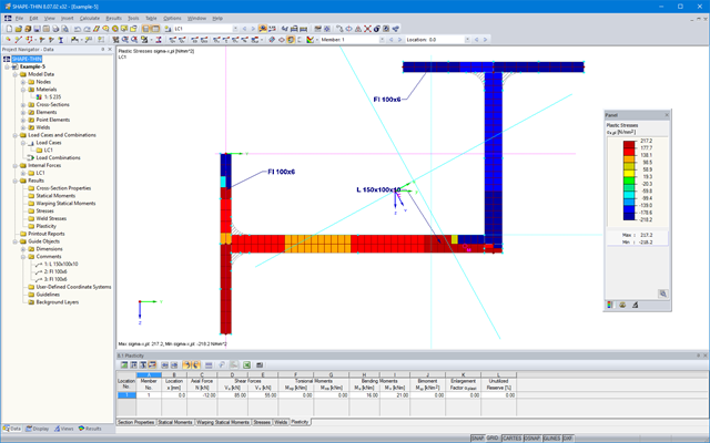
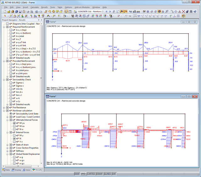
Reinforced concrete usually answers the question "How much can you carry?" simply with "Yes". Nevertheless, you need a three-dimensional moment-moment-axial force interaction diagram for the graphical output of the ultimate limit state of reinforced concrete cross-sections. The Dlubal structural analysis software offers you just that.
With the additional display of the load action, you can easily recognize or visualize whether the limit resistance of a reinforced concrete cross-section is exceeded. Since you can control the diagram properties, you can customize the appearance of the My-Mz-N diagram to suit your needs.

Do you want to determine the biaxial bending resistance of a reinforced concrete cross-section? For this, you have to activate a moment-moment interaction diagram (My-Mz diagram) first. This My-Mz diagram represents a horizontal section through the three-dimensional diagram for the specified axial force N. Due to the coupling to the 3D interaction diagram, you can also visualize the section plane there.
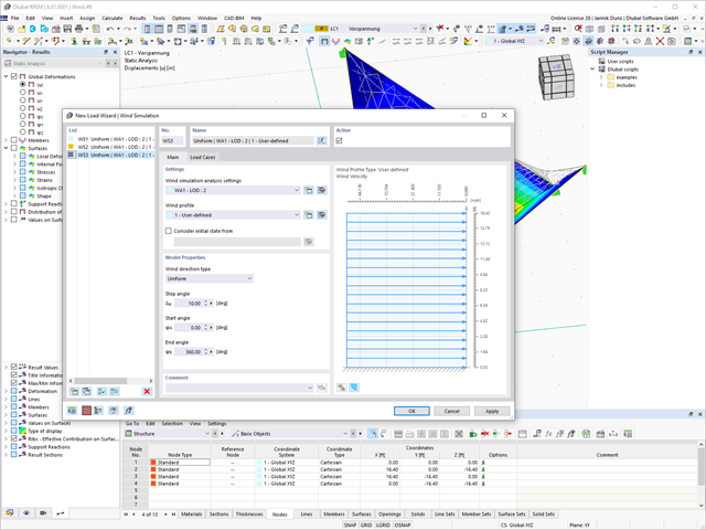
Discover the new features in RFEM and RSTAB for the determination of wind loads using RWIND:
- Useful load wizards for generating wind load cases with different flow fields in different wind directions
- Wind load cases with freely assignable analysis settings including a user-defined specification of the wind tunnel size and wind profile
- Comprehensive display of the wind tunnel with input wind profile and turbulence intensity profile
- Visualization and use of the RWIND simulation results
- Global definition of a terrain (horizontal planes, inclined plane, table)
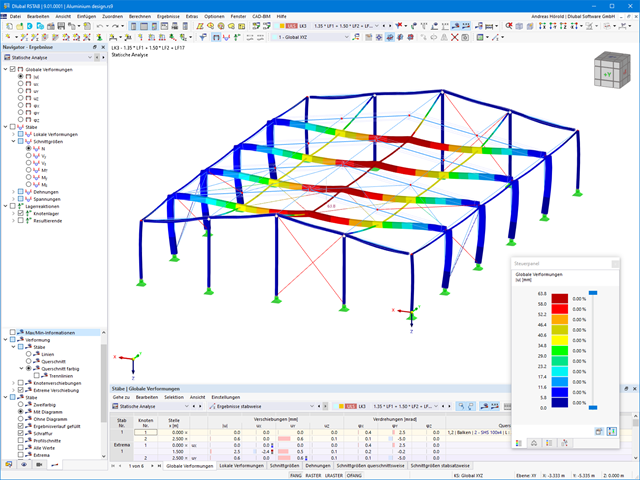
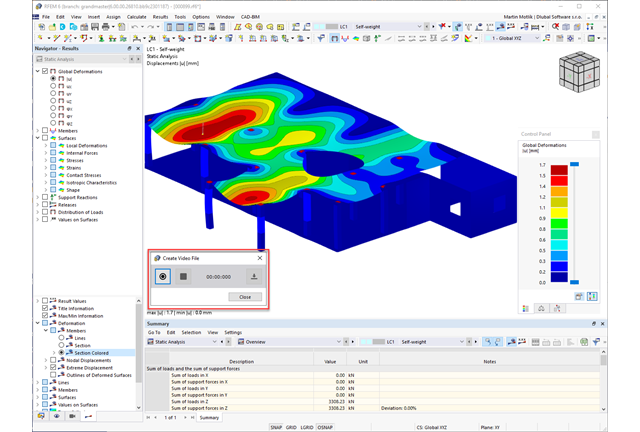
Also, on the rendered model, you see your results in a clear color display. This allows you to precisely recognize the deformation or internal forces of a member, for example. If you want to set the colors and value ranges, you can do so in the control panel.

The form-finding process gives you a structural model with active forces in the "prestress load case" This load case shows the displacement from the initial input position to the form-found geometry in the deformation results. In the force or stress-based results (member and surface internal forces, solid stresses, gas pressures, and so on), it clarifies the state for maintaining the found form. For the analysis of the shape geometry, the program offers you a two-dimensional contour line plot with the output of the absolute height and an inclination plot for the visualization of the slope situation.
Now, a further calculation and structural analysis of the entire model is performed. For this purpose, the program transfers the form-found geometry including the element-wise strains into a universally applicable initial state. You can now use it in the load cases and load combinations.

- Automatic consideration of masses from self-weight
- Direct import of masses from load cases or load combinations
- Optional definition of additional masses (nodal, linear, or surface masses, as well as inertia masses) directly in the load cases
- Optional neglect of masses (for example, mass of foundations)
- Combination of masses in different load cases and load combinations
- Preset combination coefficients for various standards (EC 8, SIA 261, ASCE 7,...)
- Optional import of initial states (for example, to consider prestress and imperfection)
- Structure Modification
- Consideration of failed supports or members/surfaces/solids
- Definition of several modal analyses (for example, to analyze different masses or stiffness modifications)
- Selection of mass matrix type (diagonal matrix, consistent matrix, unit matrix), including user-defined specification of translational and rotational degrees of freedom
- Methods for determining the number of mode shapes (user-defined, automatic - to reach effective modal mass factors, automatic - to reach the maximum natural frequency - only available in RSTAB)
- Determination of mode shapes and masses in nodes or FE mesh points
- Results of eigenvalue, angular frequency, natural frequency, and period
- Output of modal masses, effective modal masses, modal mass factors, and participation factors
- Masses in mesh points displayed in tables and graphics
- Visualization and animation of mode shapes
- Various scaling options for mode shapes
- Documentation of numerical and graphical results in printout report
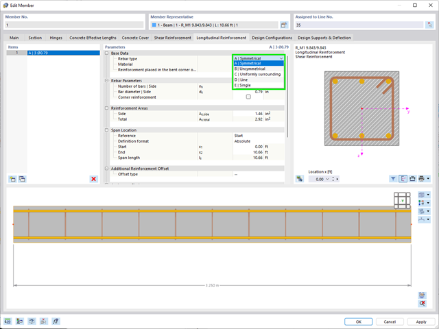
- Determination of longitudinal, shear, and torsional reinforcement
- Representation of minimum and compression reinforcement
- Determination of neutral axis depth, concrete and steel strains
- Design of member sections affected by bending about two axes
- Design of tapered members
- Design of RSECTION cross-sections (see this Product Feature)
- Determination of deformation in state II; for example, according to EN 1992‑1‑1, 7.4.3, and ACI 318‑19 24.2.3, Table 24.2.3.5
- Considering tension stiffening
- Considering creep and shrinkage
- Fatigue design according to EN 1992‑1‑1, Section 6.8 (see this Product Feature)
- Simplified fire resistance design according to EN 1992‑1‑2 for Columns (Section 5.3.2) and Beams (Section 5.6) (see this Product Feature)
- Seismic design according to EC 8 (see this Product Feature)
- Precise breakdown of reasons for failed design
- Design details of all design locations for better traceability of reinforcement determination
- Optional cross-section optimization
- Visualization of concrete section with reinforcement in 3D rendering
- Creation of 2D interaction diagrams; for example, M-N diagram
- Visualization of section resistance in 3D interaction diagram
- Output of moment-curvature diagram
- Simple definition of construction stages in the RFEM structure including visualization
- Adding, removing, modifying, and reactivating member, surface, and solid elements and their properties (for example, member and line hinges, degrees of freedom for supports, and so on)
- Automatic and manual combinatorics with load combinations in the individual construction stages (for example, to consider mounting loads, mounting cranes, and other loads)
- Consideration of nonlinear effects such as tension member failure or nonlinear supports
- Interaction with other add-ons, such as Nonlinear Material Behavior, Structure Stability, Form-Firnding, and so on.
- Display of results numerically and graphically for individual construction stages
- Detailed printout report with documentation of all structural and load data for each construction stage
RSECTION also offers everything you need in terms of overview. You can evaluate and visualize all results in an appealing numerical and graphical form. Selection functions support you in the targeted evaluation.
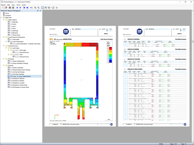
The printout report corresponds to the high standards of the FEA software RFEM and the frame analysis software RSTAB. Any modifications are updated automatically. You don't have to do anything.

- Calculation of models consisting of member, shell, and solid elements
- Nonlinear stability analysis
- Optional consideration of axial forces from initial prestress
- Four equation solvers for an efficient calculation of various structural models
- Optional consideration of stiffness modifications in RFEM/RSTAB
- Determination of a stability mode greater than the user-defined load increment factor (Shift method)
- Optional determination of the mode shapes of unstable models (to identify the cause of instability)
- Visualization of the stability mode
- Basis for determining imperfection
Also on the rendered model, you see your results in a clear color display. Thus, you can exactly recognize the rotation of a member or the stress distribution in a surface, for example. If you want to set the colors and value ranges, you can easily do so in the control panel.
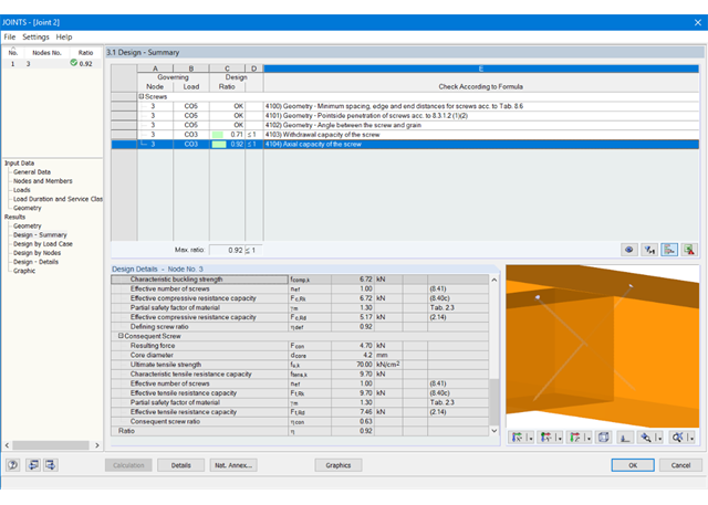
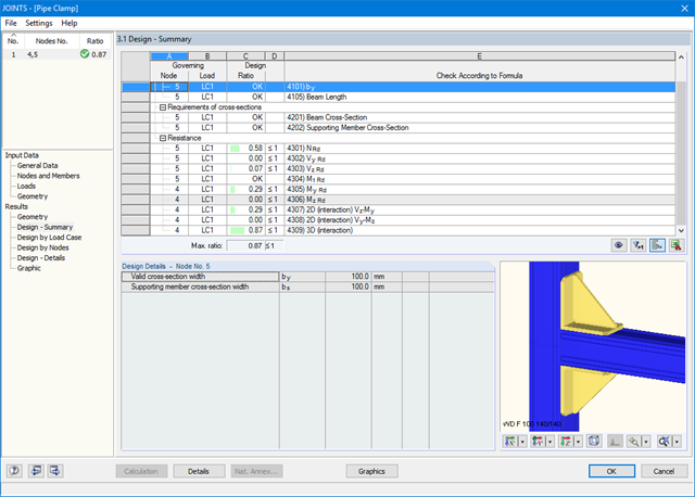
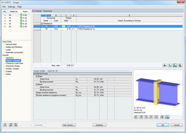
At first, the governing joint designs are arranged in groups and displayed with the basic geometry of the joint in the first result window. In the other result windows, you can see all fundamental design details.
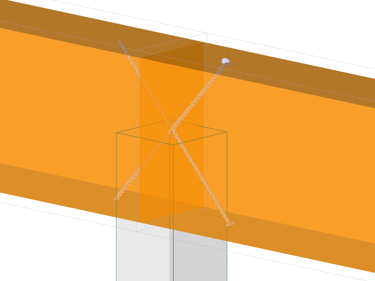
Dimensions, material properties, and welds important for the connection construction are displayed immediately and can be printed directly. Similarly, export to DXF-file is enabled. The connections can be visualized in the RF-/JOINTS Timber - Timber to Timber module as well as in RFEM/RSTAB.
All graphics can be included in the RFEM/RSTAB printout report or printed directly. Due to the scaled output, an optimal visual check is possible as early as in the design phase.
.png?mw=640&hash=c1087880acc023575381bb136280b0c348568350)
- Design of hinged connections
- Biaxial inclination of the connected member (for example, a jack rafter joint)
- Connection of any number of members on one node for the type "Main member only"
- Screw diameter 6 mm – 12 mm
- Automatic check of the minimum distance between screws
- Optional free definition of screw distances
- Transfer of eccentricity from RFEM/RSTAB
- Crosswise or parallel screw alignment
- Definition of up to 16 screws in a row
- Graphical visualization of joints in the add-on module and in RFEM/RSTAB
- Performing all required designs
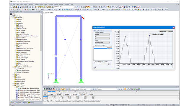
Due to the integration of RF‑/DYNAM Pro in RFEM or RSTAB, you can incorporate numeric and graphic results from RF‑/DYNAM Pro - Nonlinear Time History to the global printout report. Also, all RFEM and RSTAB options are available for a graphical visualization. The results of the time history analysis are displayed in a time history diagram.
The results are displayed as a function of time and the numerical values can be exported to MS Excel. Result combinations can be exported, either as a result of a single time step or the most unfavorable results of all time steps are filtered out.
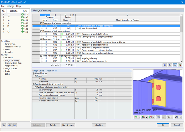
The result windows list all results of the calculation in detail. In addition, 3D graphics are created, where individual components as well as dimension lines and, for example, This allows you, for example, to display or hide the weld data. The summary shows if the individual designs have been fulfilled: The design ratio is additionally visualized with a green data bar, which turns red when the design is not fulfilled. Furthermore, the node number and the governing LC/CO/RC are displayed.
When selecting a design, the module shows the detailed intermediate results including the actions and the additional internal forces from the connection geometry. There is the option to display the results by load case and by node. The connections are represented in a realistic 3D rendering possible to scale. In addition to the main views, it is possible to show the graphics from any perspective.
You can add the graphics with dimensions and labels to the RFEM/RSTAB printout or export them as DXF. The printout report includes all input and result data prepared for test engineers. It is possible to export all tables to MS Excel or in a CSV file. A special transfer menu defines all specifications required for the export.
- Applicable for members defined as sets of members
- Separate solver that considers 7 deformation directions (ux, uy, uz, φx, φy, φz, ω) or 8 internal forces (N, Vu, Vv, Mt,pri, Mt,sec, Mu, Mv, Mω)
- Nonlinear design according to second-order analysis
- Input of imperfections
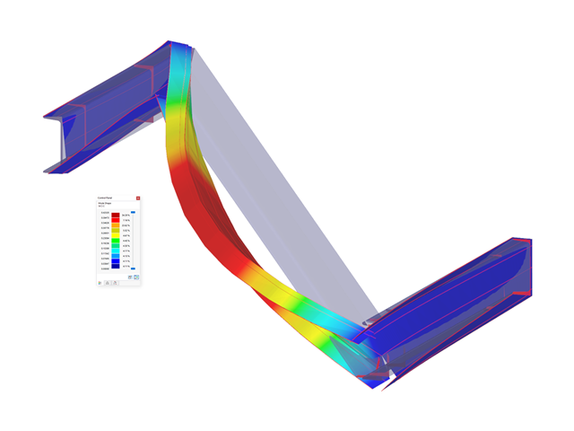
- Calculation of critical load factors and buckling mode shapes as well as the visualization of them (incl. warping)
- Integration into member design in the RF-/STEEL AISC and RF‑/STEEL EC3 add‑on modules
- Available for all thin‑walled steel cross‑sections
All results can be evaluated and visualized in an appealing numerical and graphical form. Selection functions facilitate the targeted evaluation.
The printout report corresponds to the high standards of RFEM and rstab/rstab-9/what-is-rstab RSTAB. Modifications are updated automatically.
- Full integration in RFEM/RSTAB including import of all relevant information and internal forces
- For design according to EN 1995-1-1, the following National Annexes are available:
-
 DIN EN 1995-1-1/NA:2013-08 (Germany)
 -
 ÖNORM B 1995-1-1:2015-06 (Austria)
 -
 NBN EN 1995-1-1/ANB:2012-07 (Belgium)
 -
 BDS EN 1995-1-1/NA:2012-02 (Bulgaria)
 -
 DK EN 1995-1-1/NA:2011-12 (Denmark)
 -
 SFS EN 1995-1-1/NA:2007-11 (Finland)
 -
 NF EN 1995-1-1/NA:2010-05 (France)
 -
 I S. EN 1995-1-1/NA:2010-03 (Ireland)
 -
 UNI EN 1995-1-1/NA:2010-09 (Italy)
 -
 LVS EN 1995-1-1/NA:2012-05 (Latvia)
 -
 LST EN 1995-1-1/NA:2011-10 (Lithuania)
 -
 LU EN 1995-1-1/NA:2011-09 (Luxembourg)
 -
 NEN EN 1995-1-1/NB:2007-11 (Netherlands)
 -
 NS EN 1995-1-1/NA:2010-05 (Norway)
 -
 PN EN 1995-1-1/NA:2010-09 (Poland)
 -
 NP EN 1995-1-1 (Portugal)
 -
 SR EN 1995-1-1/NB:2008-03 (Romania)
 -
 SS EN 1995-1-1 (Sweden)
 -
 STN EN 1995-1-1/NA:2008-12 (Slovakia)
 -
 SIST EN 1995-1-1/A101:2006-3 (Slovenia)
 -
 UNE EN 1995-1-1/AN:2016-04 (Spain)
 -
 CSN EN 1995-1-1/NA:2007-09 (Czech Republic)
 -
 BS EN 1995-1-1/NA:2009-10 (the United Kingdom)
 -
 CYS EN 1995-1-1/NA:2011-02 (Cyprus)
-
- Extensive material library in compliance with the EN, SIA, and DIN standards
- Design of circular, rectangular, and user-defined composite cross-sections (also hybrids)
- Specific classification of a structure in service classes (SECL) and actions in load duration classes (LDC)
- Design of members and sets of members
- Stability analysis according to the Equivalent Member Method or the second-order analysis
- Determination of governing internal forces
- Icon providing information about successful or failed design
- Visualization of the design criterion on RFEM/RSTAB model
- Automatic cross-section optimization
- Parts lists and quantity surveying
- Data export to MS Excel
- Free configuration of charring time and charring rates, as well as free choice of charring sides for fire design
- Fire resistance designs in the selected standard according to:
-
 EN 1995-1-2
 -
SIA 265:2012 + SIA 265-C1:2012
-
to DIN 4102-22:2004
-
- Import of buckling lengths from the RF-STABILITY/RSBUCK add-on module
- Design of tapered members according to the previously defined cut-to-grain angle
- Ridge design and analysis of transversal tension stresses for defined ridges
- Design of curved members and sets of members
The existing loading is compared to the load resistances stored in the database. The program also performs the interaction of internal forces M, N, and Q.
After the design, all results are displayed in clearly arranged result tables; for example, by load case or by node.
You can visualize the joints graphically in the add-on module or in RFEM/RSTAB. In addition to the input and result data, including design details displayed in tables, you can add all graphics into the printout report. This way, comprehensible and clearly arranged documentation is guaranteed.
After the design, all results are displayed in clearly arranged result tables; for example, by load case or by node. The governing internal forces are compared with the limit values listed in the DSTV guideline.
You can visualize the joints graphically in the add-on module or in RFEM/RSTAB. In addition to the input and result data, including design details displayed in tables, you can add all graphics into the printout report. This way, comprehensible and clearly arranged documentation is guaranteed.
- Automatic consideration of masses from self-weight
- Direct import of masses from load cases or load combinations
- Optional definition of additional masses (nodal, linear, surface masses, as well as inertia masses)
- Combination of masses in different mass cases and mass combinations
- Preset combination coefficients according to EC 8
- Optional import of normal force distributions (in order to consider prestress, for example)
- Stiffness modification (for example, deactivated members or stiffnesses can be imported from RF-/CONCRETE)
- Consideration of failed supports or members
- Definition of several natural vibration cases (for example, to analyze different masses or stiffness modifications)
- Results of eigenvalue, angular frequency, natural frequency, and period
- Determination of mode shapes and masses in nodes or FE mesh points
- Results of modal masses, effective modal masses, and modal mass factors
- Visualization and animation of mode shapes
- Various scaling options for mode shapes
- Documentation of numerical and graphical results in the printout report
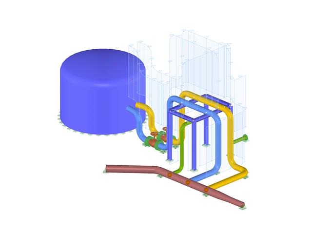
- Graphical input of piping systems and piping components
- Illustrative visualization of piping systems and piping components in RFEM graphic window
- Comprehensive libraries for piping cross‑sections and materials
- Comprehensive libraries for flanges, reducers, tees, and expansion joints
- Consideration of piping structure (insulation, lining, tin‑plate)
- Automatic calculation of stress intensification factors and flexibility factors
- Specific piping action categories for load cases
- Optional automatic combinatorics of load cases
- Consideration of material properties (modulus of elasticity, coefficient of thermal expansion) either during operating temperature (default setting) or during reference (assembly) temperature of material
- Consideration of strain and uplift due to pressure (Bourdon effect)
- Interaction between the supporting structure and the piping system
- Full integration in RFEM/RSTAB including import of all relevant information and internal forces
- Design of members and continuous members for tension, compression, bending, shear, and combined internal forces
- Stability analysis for lateral-torsional buckling and buckling according to the equivalent member method or the second order analysis
- Serviceability limit state design by limitation of deflections
- Free configuration of charring time and charring rates, as well as free choice of charring sides for fire design
- South African material library and cross‑section library
- User-defined entry of rectangular and circular cross-sections
- Cross-section optimization with optional transfer to RFEM/RSTAB
- Optional import of effective lengths from the RSBUCK or RF‑STABILITY add‑on module
- Detailed result documentation including references to design equations of the used standard
- Various filter and sorting options of results including result lists by member, cross-sections, x-location, or by load case, load and result combination
- Consideration of moisture service conditions
- Visualization of the design criterion on the RFEM/RSTAB model
- Data export to MS Excel
- Design of members and continuous members for tension, compression, bending, shear, and combined internal forces
- Stability analysis for lateral-torsional buckling and buckling according to the equivalent member method or the second order analysis
- Serviceability limit state design by limitation of deflections
- Free configuration of charring time and charring rates, as well as free choice of charring sides for fire design
- Design of tapered and curved beams consisting of glulam timber
- Material and cross‑section library based on the Canadian standard
- User-defined entry of rectangular and circular cross-sections
- Automatic cross-section optimization
- Optional import of buckling lengths from the RF-STABILITY/RSBUCK module
- Detailed result documentation including references to design equations of the used standard
- Various filtering and sorting options of results
- Consideration of moisture service conditions
- Visualization of design criterion on RFEM/RSTAB model
- Data export to MS Excel
- Units metric and imperial
After the calculation, the module shows clearly arranged tables listing the required reinforcement and the results of the serviceability limit state design. All intermediate values are included in a comprehensible manner. In addition to the tables, current stresses and strains in a cross‑section are represented graphically.
The reinforcement proposals of the longitudinal and the shear reinforcement, including sketches, are documented in accordance with current practice. It is possible to edit the reinforcement proposal and to adjust, for example, the number of members and the anchorage. The modifications will be updated automatically.
A concrete cross‑section, including reinforcement, can be visualized in a 3D rendering. This way, the program provides an optimal documentation option to create reinforcement drawings, including steel schedule.
Crack width analyzes are performed using the selected reinforcement of internal forces in the serviceability limit state. The result output covers steel stresses, the minimum reinforcement, limit diameters, and the maximum bar spacing, as well as crack spacing and the maximum crack widths.
As a result of the nonlinear calculation, there are the ultimate limit states of the cross‑section with defined reinforcement (determined linear elastically) as well as effective deflections of the member considering stiffness in cracked state.