


The "Transient Flow" calculation can be set on the "General" tab of the "Simulation Parameters" dialog box. There you can also choose whether to save the data needed to continue the calculation after reopening the model. It could be useful, but it produces large files.
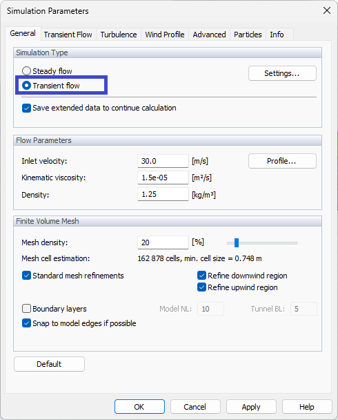
On the "Transient Flow" tab, the parameters of the transient flow simulation can be defined.

Initial Condition
The initial condition for the transient calculation is set in this section. By default, the steady flow is calculated first. The results are then used as the initial field for the transient calculation. You can also define a number of iterations for this steady flow calculation.
When calculating the transient flow, it is important to set the initial condition correctly. An improperly set initial condition may cause either instability of the calculation or an unnecessarily long calculation time before the flow field stabilizes at the correct values. RWIND 3 uses its steady-flow solver with a low number of iterations to calculate the initial condition. This means that when calculating the transient flow, the steady-flow calculation of the initial condition is started first, and as soon as it is finished, the transient calculation is started automatically.
Boundary Conditions
A time-varying boundary condition could be defined at the tunnel inlet. Checking this option, the defined steady profiles for velocity and turbulence quantities are deleted. A new dialog box opens.

The values of the transient boundary condition are defined on a set of points lying on the tunnel inlet boundary. These points are defined in the "Definition points of the boundary condition" section. It is possible to define them manually or to import them from a point cloud. The point cloud can be created using the New point cloud graphically… function. Only y,z coordinates are considered, so the x-coordinate can be arbitrary. The points must be inside the tunnel and cannot be collinear (in a line only). Therefore, the rectangle type of the point cloud is the most suitable.
The time history of the selected quantity (e.g. velocity components) is then defined in the "Values in time in selected points" section, with the specified values valid for the currently selected point or for multiple selected points simultaneously. The points can be checked in the first section or selected by the graphical tool in the last section. For the DDES turbulence model, only velocity components can be defined. For URANS, time-variable k, epsilon or omega can be defined, too.
The third section shows the time history of the selected quantity for the selected points.
All points and values can be also pasted from clipboard or the whole BC can be imported via XML file (this will be explained later).
The initial time of the condition must be equal to or less than the beginning of the transient calculation (0, when starting the transient calculation, or equal to or less than the current simulation time, when continuing transient calculation). The times can be offset to 0 or another time, when needed, by the “Import, Export and Other Functions...” button.
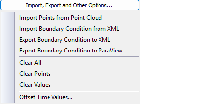
Both the points and the values of the transient condition can be imported (or exported) from (or to) an XML file, using the menu under the "Import, Export and Other Options" button.
When the time interval of BC is shorter than the time interval of the calculation, the last value is maintained until the end of the calculation.
Transient Flow Calculation and Results
In this section, you can set the calculation time and the optimum time steps for saving the transient results. The default setting is recommended; more experienced users can change this setting at their discretion, but it is important to realize that inappropriate settings may cause a large amount of data to be stored on disk (tens or hundreds of GB), which may significantly slow down the calculation as well as the subsequent work with the program.
The "Simulation time" is the real time of the wind flow we want to calculate. The default value (given by the automatic setting) corresponds to approximately 10 times the time required for the wind to pass through the entire length of the tunnel at a given inlet speed.
The start time for saving results is the time from which transient results are to be saved. It allows you to avoid storing data in the initial phase of the calculation, in which the numerical solution does not yet converge to the correct values. A time step can be defined, and based on the above inputs, the number of time steps is calculated.
A special option for RFEM 6 or RSTAB 9 program for structural analysis defines which time step will be considered as the "master time step". By default, the "Last Time Layer" is set as the master time layer, but you can change this value either on this tab or from the pop-up menu that is available on the "Edit Bar" after the calculation.
When available, information about existing results is provided: achieved simulation time and number of calculated steps (DTL).
Transient Calculation Options
When clicking on the Other Options button, a new dialog box appears:
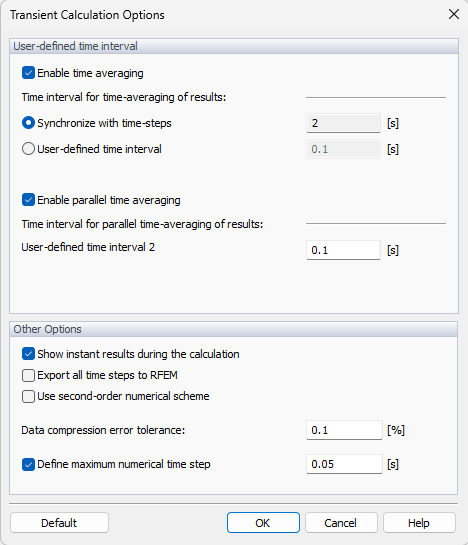
Time Averaging of Results
The instant results can be averaged directly in OpenFOAM across a moving averaging window defined by a time interval. The time interval can be synchronized with the saving time step or arbitrary.
For very special purposes, such as calculation of cp,1 and cp,10 pressure coefficients, a parallel averaging is possible. Enabling this option, the results calculated by OpenFOAM are averaged independently by two different moving windows. After the calculation, two sets of results (surface pressure, cp and flow field pressure) are available.
Other Options
The "Show instant results during calculation" option allows enabling/disabling the display of results in time steps during the calculation.
The "Export all time steps to RFEM" option allows you to save/transfer the results of all saved time steps to RFEM. This affects also the output, when exporting results directly from RWIND (either to ParaView or all results).
The "Use second-order numerical scheme" check box controls which numerical scheme is used for divergence terms (fluxes). It is not activated by default, so the calculation is carried out according to the first order. If the check box has been selected, the solution is performed according to the second order.
Next, there is a parameter for setting the "Data compression error tolerance" when compressing the data of the transient results: As the data of transient results can be huge, RWIND 3 allows for the compression of the data, which can still entail a certain error into some time layers. This tolerance indicates how much the value at a given point can differ from the value obtained from the calculation.
The default tolerance is set to 0.1%, which means the value ε = 0.001 · (Vmax - Vmin), where Vmax and Vmin are the maximum and minimum values in the whole domain. If the tolerance is set to zero, no compression will be performed, and all values in all time steps correspond to the values obtained from the calculation.
Lastly, there is an option to limit the numerical time step. RWIND uses the adaptive time step in order to keep the shortest possible calculation time while fulfilling the needed stability criteria. With coarse spatial meshing, this can result in coarse time steps. If needed, prescribing the maximum numerical time step limits the length of the time steps. However, the calculation can take longer then.