92 Wyniki
Wyświetl wyniki:
Sortuj według:

Za pomocą interfejsu SDNF można importować i eksportować dane, takie jak materiały, przekroje, pręty i powierzchnie w programach RFEM 6 i RSTAB 9. Umożliwia to wymianę danych z programami, takimi jak Tekla Structures lub Advance Steel, opartą na plikach.
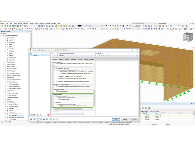
Teraz w rozszerzeniu Projektowanie konstrukcji betonowych można wymiarować elementy wykonane z betonu zbrojonego włóknami zgodnie z wytyczną "DAfStb Steel Fiber-Reinforced Concrete".
Ta opcja jest dostępna dla obliczeń zgodnie z EN 1992-1-1. Obliczenia zgodnie z wytyczną DAfStb są przeprowadzane po przypisaniu betonu typu "Fibrobeton" do elementu konstrukcyjnego z betonu zbrojonego.
Przejdź do filmu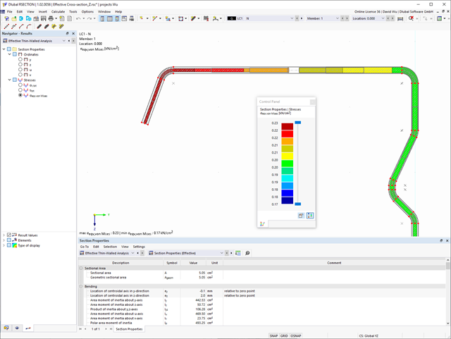
Przekroje efektywne jest rozszerzeniem programu RSECTION do określania właściwości przekrojów. W porównaniu z modułem dodatkowym RF-/STEEL Cold-Formed Sections dla programu RFEM 5/RSTAB 8, do Przekrojów efektywnych dodano następujące nowe funkcje:
- Uwzględnienie efektów wyboczenia dystorsyjnego przekrojów metodą wartości własnych
- Definiowanie usztywnień i paneli wyboczeniowych nie jest już konieczne
- Graficzne wyświetlanie naprężeń jednostkowych
- Opcjonalna ręczna definicja punktów naprężeniowych
- 002171
- Ogólne informacje
- Projektowanie konstrukcji stalowych RFEM 6
- Projektowanie konstrukcji stalowych RSTAB 9
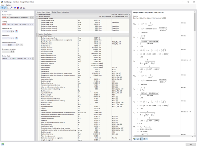
W porównaniu z modułem dodatkowym RF-/STEEL EC3 (RFEM 5/RSTAB 8) do rozszerzenia Wymiarowanie stali dla programu RFEM 6/RSTAB 9 dodano następujące nowe funkcje:
- Oprócz Eurokodu 3, uwzględnione zostały inne międzynarodowe normy (np. AISC 360, CSA S16, GB 50017, SP 16.13330)
- Berücksichtigung der Feuerverzinkung (DASt-Richtlinie 027) beim Brandschutznachweis nach EN 1993-1-2
- Opcja wprowadzania żeber usztywniających, które można uwzględnić w analizie wyboczenia
- Wyboczenie skrętne można również sprawdzić w przypadku przekrojów zamkniętych (np. istotne dla smukłych, wysokich prostokątnych przekrojów zamkniętych)
- Automatyczne wykrywanie prętów lub zbiorów prętów ważnych dla obliczeń (np. automatyczna dezaktywacja prętów z nieaktualnym materiałem lub prętów już zawartych w zbiorze prętów)
- Możliwość dostosowania ustawień obliczeniowych indywidualnie dla każdego pręta
- Graficzne przedstawienie wyników w przekroju brutto lub przekroju efektywnym
- Wyświetlanie odpowiednich wzorów użytych do sprawdzania warunków nośności (w tym odniesienie do zastosowanego równania z normy)

- 002165
- Ogólne informacje
- Skręcanie skrępowane (7 stopni swobody) RFEM 6
- Skręcanie skrępowane (7 stopni swobody) RSTAB 9
W porównaniu z modułem dodatkowym RF-/STEEL Warping Torsion (RFEM 5/RSTAB 8) do rozszerzenia Skręcanie skrępowane (7 DOF) dla programu RFEM 6/RSTAB 9 dodano następujące nowe funkcje:
- Pełna integracja ze środowiskiem RFEM 6 i RSTAB 9
- Siódmy stopień swobody jest bezpośrednio uwzględniany w obliczeniach prętów w programie RFEM/RSTAB na całym układzie
- Nie ma już potrzeby definiowania warunków podparcia lub sztywności sprężystej do obliczeń w uproszczonym układzie zastępczym
- Możliwość łączenia z innymi rozszerzeniami, na przykład do obliczania obciążeń krytycznych dla wyboczenia skrętnego i zwichrzenia z analizą stateczności
- Brak ograniczeń dla stalowych przekrojów cienkościennych (możliwe jest również obliczenie momentu krytycznego, na przykład dla belek o masywnych przekrojach drewnianych)
- 002169
- Ogólne informacje
- Analiza naprężeniowo-odkształceniowa RFEM 6
- Analiza naprężeniowo-odkształceniowa RSTAB 9
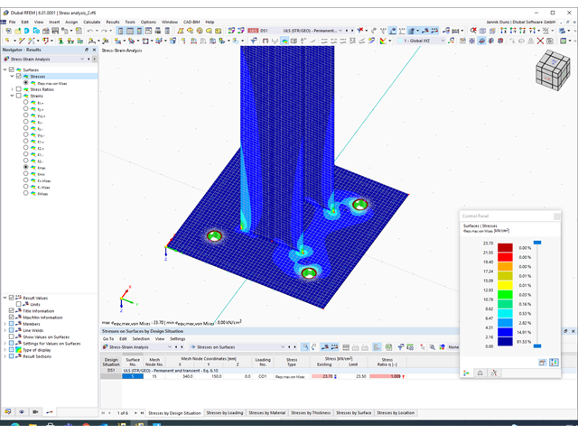
W porównaniu z modułem dodatkowym RF-/STEEL (RFEM 5/RSTAB 8) do rozszerzenia Analiza naprężeniowo-odkształceniowa dla programu RFEM 6/RSTAB 9 dodano następujące nowe funkcje:
- Możliwość analizy prętów, powierzchni, brył, spoin (połączenia spawane liniowo między dwiema i trzema powierzchniami z późniejszym obliczaniem naprężeń)
- Wyświetlanie naprężeń, stopni naprężeń, zakresów naprężeń i odkształceń
- Naprężenie graniczne w zależności od przydzielonego materiału lub danych wejściowych zdefiniowanych przez użytkownika
- Indywidualne określenie wyników do obliczeń poprzez dowolnie przydzielane typów ustawień
- Szczegóły dla wyników niemodalnych z wyświetlaniem przygotowanego wzoru i dodatkowym wyświetlaniem wyników na poziomie przekroju prętów
- Możliwość wygenerowania zastosowanych wzorów do kontroli obliczeń
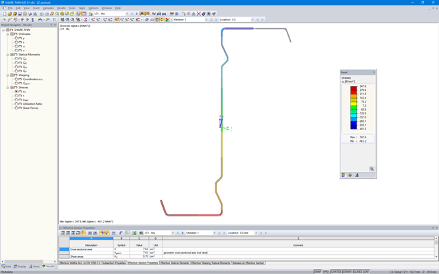
SHAPE-THIN określa przekroje efektywne zgodnie z EN 1993-1-3 i EN 1993-1-5 dla profili formowanych na zimno. Opcjonalnie można sprawdzić warunki geometryczne pod kątem możliwości zastosowania normy określonej w EN 1993-1-3, rozdział 5.2.
Efekty miejscowego wyboczenia płyty są uwzględniane zgodnie z metodą zmniejszonej szerokości, a ewentualne wyboczenie usztywnień (niestateczność) jest uwzględniane w przypadku przekrojów usztywnionych zgodnie z EN 1993-1-3, rozdział 5.5.
W celu zoptymalizowania przekroju efektywnego, opcjonalnie można przeprowadzić obliczenia iteracyjne.
Przekroje efektywne można wyświetlić w postaci graficznej.
Więcej informacji na temat wymiarowania profili zimnogiętych w modułach SHAPE-THIN i RF-/STEEL Cold-Formed Sections można znaleźć w artykule technicznym "Wymiarowanie przekrojów ceowych cienkościennych zgodnie z EN 1993-1-3".
Wymiarowanie przekroju ceowego cienkościennego zgodnie z EN 1993-1-3 Więcej o RF-STEEL Cold-Formed Sections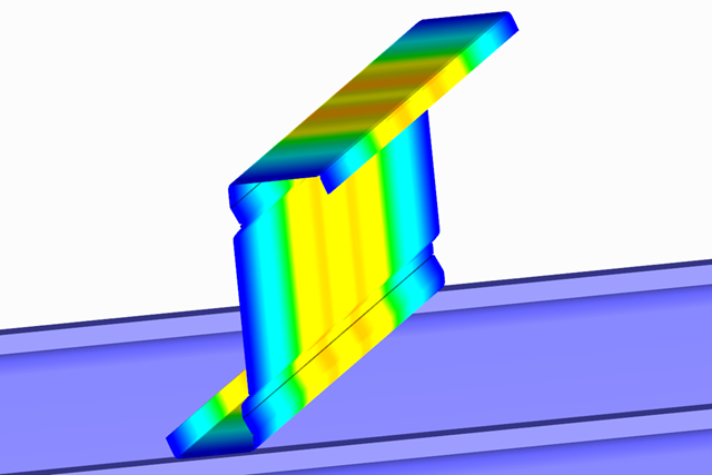
- Dostępne dla przekrojów L, Z, C, CL, ceowników, kształtowników kapeluszowych dostępnych w bazie danych przekrojów, a także dla ogólnych formowanych na zimno przekrojów (nieperforowanych) SHAPE-THIN-9 profile
- Określenie przekroju efektywnego z uwzględnieniem wyboczenia lokalnego i wyboczenia dystorsyjnego
- Obliczenia przekroju, stanu granicznego użytkowalności i stateczności według EN 1993-1-3
- Obliczanie lokalnych sił poprzecznych dla środników bez usztywnienia
- Dostępne dla wszystkich załączników krajowych zawartych w RF-/STEEL EC3
- Rozszerzenie modułu RF-/STEEL Warping Torsion (wymagana licencja) dla analizy stateczności według analizy drugiego rzędu jako analiza naprężeń z uwzględnieniem 7th stopnia swobody (skręcanie)
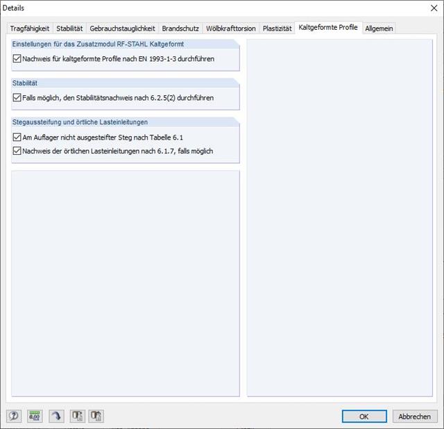
Ponieważ RF-/STEEL Cold-Formed Sections jest w pełni zintegrowany z RF-/STEEL EC3, dane są wprowadzane w taki sam sposób, jak w przypadku każdej konstrukcji w tym module. W oknie dialogowym Szczegóły należy tylko wybrać opcję wymiarowania profili zimnogiętych.
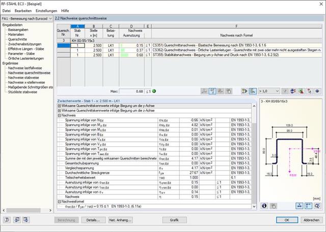
Wyniki obliczeń są wyświetlane w RF-/STEEL EC3 w zwykły sposób.
Odpowiednie okna wyników zawierają, między innymi, efektywne właściwości przekroju wywołane działaniem siły osiowej N, momentu zginającego My, momentu zginającego Mz, sił wewnętrznych oraz podsumowanie obliczeń.
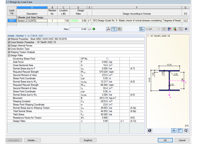
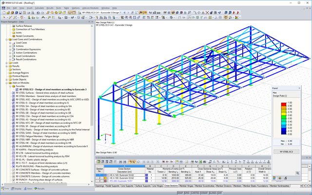
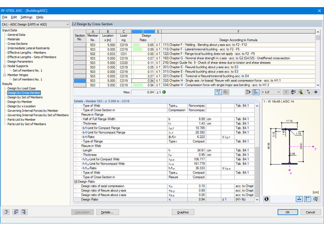
Dzięki zintegrowanemu rozszerzeniu modułu RF-/STEEL Warping Torsion, możliwe jest przeprowadzenie obliczeń zgodnie z Design Guide 9 w RF-/STEEL AISC.
Obliczenia są przeprowadzane z 7 stopniami swobody zgodnie z teorią skręcania skrępowanego i umożliwiają realistyczne obliczenia stateczności z uwzględnieniem skręcania.
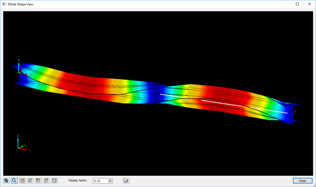
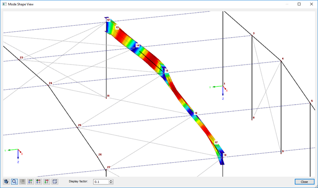
Definiowanie krytycznego momentu wyboczeniowego odbywa się w module RF-/STEEL AISC za pomocą solwera wartości własnych, który umożliwia dokładne określenie krytycznego obciążenia wyboczeniowego.
Solwer wartości własnych pokazuje okno z grafiką wartości własnych, które umożliwia sprawdzenie warunków brzegowych.
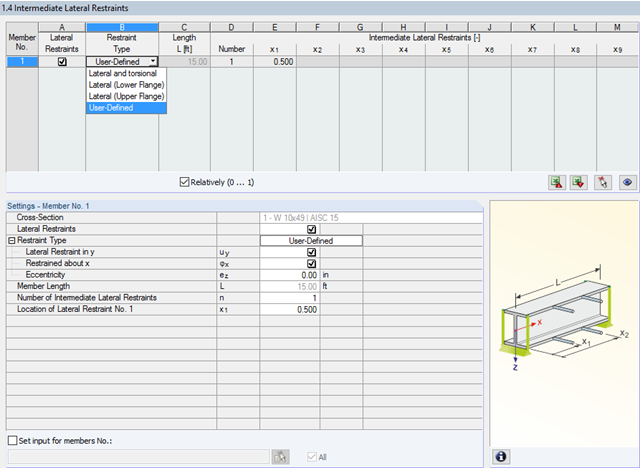
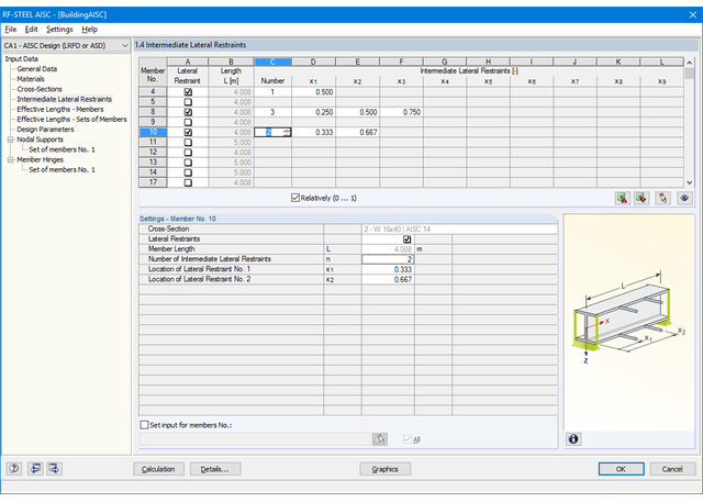
W programie STEEL AISC możliwe jest uwzględnienie pośrednich podpór bocznych w dowolnym miejscu. Na przykład, możliwa jest stabilizacja tylko górnej półki.
Ponadto można przypisać boczne podpory pośrednie zdefiniowane przez użytkownika; na przykład pojedyncze sprężyny obrotowe i sprężyny translacyjne w dowolnym miejscu przekroju.
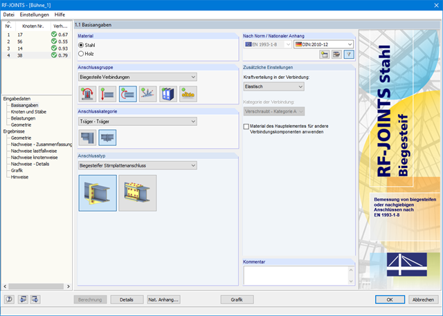
Po uruchomieniu modułu należy wybrać grupę połączeń (połączenia sztywne), a następnie kategorię i typ połączenia (styk z blachą czołową lub styk z nakładkami). Kolejnym krokiem jest wybranie w modelu RFEM/RSTAB węzłów przeznaczonych do obliczeń. RF-/JOINTS Steel - Rigid automatycznie rozpoznaje pręty połączenia i określa na podstawie ich położenia, czy są to słupy czy belki. Na tym etapie użytkownik może wprowadzić własne ustawienia.
W przypadku, gdy określone pręty mają zostać wyłączone z obliczeń, można je dezaktywować. Konstrukcyjnie podobne połączenia mogą być projektowane jednocześnie dla kilku węzłów. Należy wybrać przypadki obciążeń, kombinacje obciążeń i kombinacje wyników. Alternatywnie, można ręcznie wprowadzić przekrój i obciążenie. W ostatniej tabeli wejściowej, połączenie jest konfigurowane krok po kroku.
_(2).png?mw=640&hash=0414bfe44045fc798e3774a0173332ca37424418)
Ogólne informacje
- Połączenie typu belka-słup: możliwość wykonania zarówno w postaci połączenia belki z półką słupa, jak również w postaci połączenia słupa z półką belki
- Połączenie typu belka-belka: wymiarowanie połączeń belek możliwe zarówno jako połączenia przenoszące moment z blachą czołową, jak i sztywne połączenia nakładkowe
- Możliwość automatycznego eksportu danych modelu i obciążeń z programu RFEM lub RSTAB
- Rozmiary śrub od M12 do M36 z klasami wytrzymałości 4.6, 4.8, 5.6, 5.8, 6.8, 8.8 i 10.9 (o ile dana klasa wytrzymałości jest dostępna w wybranym załączniku krajowym)
- Niemal dowolne rozstawy śrub i odległości od krawędzi (program sprawdza dopuszczalne rozstawy)
- Wzmocnienie belek za pomocą skosów lub usztywnień na górnej i dolnej powierzchni
- Połączenie z blachą czołową wystającą lub niewystającą
- Możliwa jest kombinacja na samo zginanie, samą siłę osiową (styk rozciągany) lub na kombinację siły osiowej i zginania
- Obliczanie sztywności połączeń i sprawdzanie, czy istnieje połączenie przegubowe, półsztywne czy sztywne
Połączenie z blachą czołową w konfiguracji belka-słup
- Połączone belki lub słupy mogą być wzmocnione jednostronnie za pomocą skosów lub też jedno- lub dwustronnie przy użyciu żeber usztywniających
- Szeroki wybór dostępnych usztywnień połączenia (np. pełne lub niekompletne żebra środnika)
- Możliwość zastosowania do dziesięciu śrub w poziomie i czterech śrub w pionie
- Element przyłączany może być profilem dwuteowym o stałym lub zmiennym przekroju
- Wyk. przekroju:
- Nośność połączonej belki (np. nośność blachy środnika przy ścinaniu i rozciąganiu)
- Nośność blachy czołowej belki (np. króciec teowy poddany rozciąganiu)
- Nośność spoin blachy czołowej
- Nośność słupa w obszarze połączenia (np. pas słupa poddany zginaniu - króciec teowy)
- Wszystkie obliczenia są przeprowadzane w oparciu o normę EN 1993-1-8 lub EN 1993-1-1.
Przegubowe połączenie z blachą czołową
- Dwa lub cztery pionowe rzędy śrub i maks. 10 poziomych rzędów śrub
- Łączone belki mogą być wzmocnione za pomocą skosów po jednej stronie lub za pomocą żeber usztywniających po jednej lub obu stronach
- Elementy przyłączane mogą być profilami dwuteowymi o stałym lub zmiennym przekroju
- Wyk. przekroju:
- Nośność łączonych belek (np. nośność blach środnika przy ścinaniu i rozciąganiu)
- Nośność blach czołowych belek (np. króciec teowy poddany rozciąganiu)
- Nośność spoin blach czołowych
- Nośność śrub w blasze czołowej (kombinacja rozciągania i ścinania)
Sztywne połączenie nakładkowe
- W połączeniu z blachą pasów możliwość zastosowania nawet do 10 rzędów śrub
- W przypadku połączenia ze środnikiem i blachą można zastosować do dziesięciu rzędów śrub w kierunku pionowym i poziomym
- Materiał nakładek może być inny niż materiał belek
- Wyk. przekroju:
- Nośność łączonych belek (np. przekrój netto w obszarze rozciągania)
- Nośność blach nakładkowych (np. przekrój netto poddany rozciąganiu)
- Nośność pojedynczych śrub i grup śrub (np. nośność na ścinanie pojedynczej śruby)
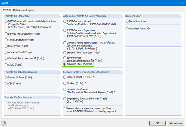
Podczas wymiany danych z Advance Steel przy użyciu plików *.smlx, interfejs jest wykrywany automatycznie. Oznacza to, że pliki *.smlx mogą być tworzone nawet wtedy, gdy nie jest zainstalowana żadna wersja Advance Steel.
- Ogólna analiza naprężeniowa
- Automatyczny import sił wewnętrznych z programu RFEM/RSTAB
- Pełne graficzne i numeryczne przedstawianie naprężeń i stopni wykorzystania przekroju w programie RFEM/RSTAB
- Szeroki zakres opcji umożliwiających dostosowywania sposobu wyświetlania wyników
- Swoboda obliczeń dzięki możliwości wykorzystania różnych przypadków obliczeniowych
- Przejrzyste tabele wyników dla szybkiego ich przeglądania po zakończeniu obliczeń
- Wysoka wydajność pracy dzięki minimalnej ilości danych wejściowych
- Elastyczność dzięki szczegółowym opcjom ustawień dla podstawy i zakresu obliczeń
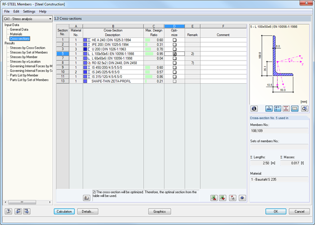
- Optymalizacja przekroju
- Transfer zoptymalizowanych przekrojów do RFEM/RSTAB
- Wymiarowanie dowolnego przekroju cienkościennego w SHAPE-THIN
- Odwzorowanie wykresu naprężeń na przekroju
- Wyznaczanie naprężeń normalnych, ścinających i równoważnych
- Wyniki naprężeń poszczególnych typów sił wewnętrznych
- Szczegółowe przedstawienie naprężeń we wszystkich punktach naprężeniowych
- Wyznaczanie największego Δσ dla każdego punktu naprężenia (na przykład do obliczeń zmęczenia)
- Wyświetlanie w kolorze naprężeń i stopni wykorzystania w celu szybkiego przeglądu stref krytycznych lub przewymiarowanych
- Wykaz materiałów według prętów i zbiorów prętów
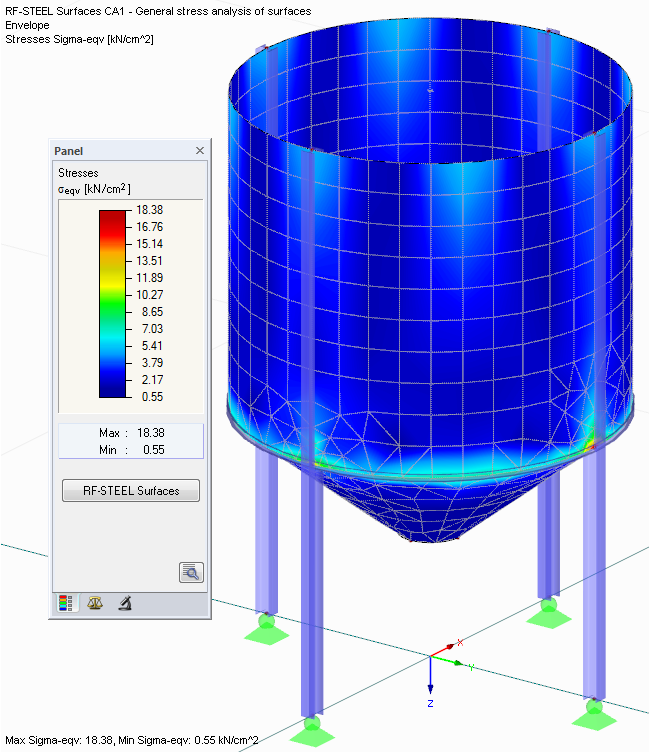
- Wyznaczanie naprężeń głównych i podstawowych, naprężeń membranowych i stycznych oraz naprężeń zastępczych i zastępczych naprężeń membranowych
- Analiza naprężeń dla elementów konstrukcyjnych o dowolnym kształcie
- Obliczanie naprężeń zastępczych według różnych metod:
- Hipoteza energii odkształcenia (von Mises)
- Hipoteza naprężeń stycznych (Tresca)
- Hipoteza naprężenia normalnego (Rankine)
- Hipoteza głównego odkształcenia (Bach)
- Możliwość optymalizacji grubości powierzchni i transferu danych do programu RFEM
- Obliczenia w stanie granicznym użytkowalności poprzez sprawdzanie przemieszczeń powierzchni
- Szczegółowe wyniki dla różnych składników naprężeń i stopni wykorzystania w tabelach i w grafice
- Funkcja filtrowania tabeli dla powierzchni, linii i węzłów
- Poprzeczne naprężenia styczne według Mindlina, Kirchhoffa lub zdefiniowane przez użytkownika
- Wykaz materiałów dla analizowanych powierzchni
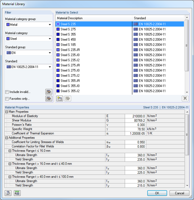
Aby ułatwić wprowadzanie danych, wstępnie ustawione są powierzchnie, pręty, zbiory prętów, materiały, grubości powierzchni i przekroje. Elementy można wybierać graficznie za pomocą funkcji [Wybierz]. Program zapewnia dostęp do globalnych bibliotek materiałów i przekrojów.
Przypadki obciążeń, kombinacje obciążeń i kombinacje wyników można łączyć w różne przypadki obliczeniowe.
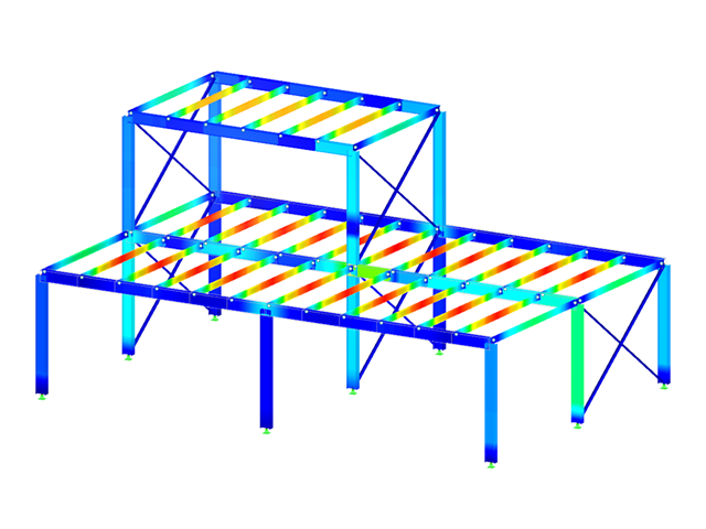
Połączenie elementów powierzchniowych i prętowych oraz oddzielne obliczenia umożliwiają modelowanie i analizowanie tylko krytycznych części, takich jak połączenia ram, za pomocą elementów powierzchniowych. Pozostałe części modelu można przeprowadzić za pomocą analizy prętów.
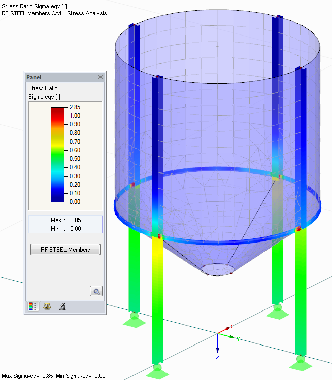
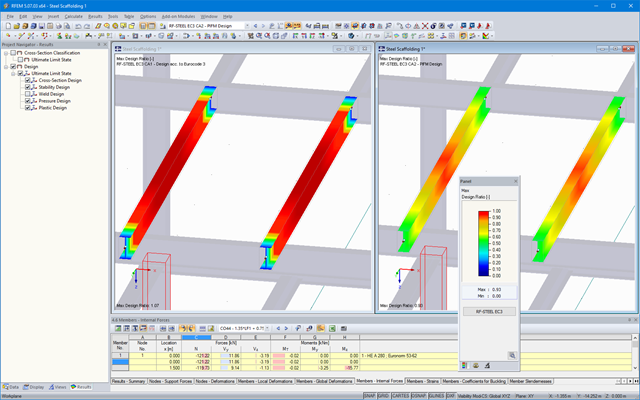
Po zakończonych obliczeniach, maksymalne naprężenia oraz stopnie wytężenia są wyświetlane wg przekrojów, prętów/powierzchni, zbiorów prętów lub położenia x wzdłuż elementu. Oprócz wartości wyników w formie tabelarycznej wyświetlana jest również odpowiednia grafika przekroju z punktami naprężeniowymi, wykresem naprężeń i wartościami. Stopień wytężenia można wyznaczyć w odniesieniu do dowolnego rodzaju naprężenia. Aktualnie wybrana lokalizacja na elemencie zostanie wyróżniona na modelu analitycznym w programie RFEM/RSTAB.
Ponadto wszystkie wyniki modułu RF-/STEEL można wyświetlać w oknie roboczym programu RFEM/RSTAB. Istnieje możliwość indywidualnego dostosowania kolorów wyświetlania wykresów oraz wartości.
Wykresy pokazujące rozkład wyników na pręcie lub zbiorze prętów pozwalają na szczegółową ocenę wyników. Ponadto można otworzyć odpowiednie okno dialogowe dla każdej lokalizacji, aby sprawdzić właściwości przekroju i składowe naprężeń w dowolnym punkcie naprężeniowym. Można wydrukować odpowiadającą temu grafikę wraz ze wszystkimi szczegółami dotyczącymi sprawdzanych warunków nośności.
- Import materiałów, przekrojów i sił wewnętrznych z RFEM/RSTAB
- Wymiarowanie stali dla przekrojów cienkościennych zgodnie z EN 1993‑1‑1: 2005 i EN 1993‑1‑5: 2006
- Automatyczna klasyfikacja przekrojów według EN 1993-1-1:2005 + AC:2009, rozdział 5.5.2 oraz EN 1993-1-5:2006, rozdział 4.4 (przekrój klasy 4) z możliwością określenia szerokości efektywnej zgodnie z załącznikiem E dla naprężeń poniżej fy
- Integracja parametrów dla następujących załączników krajowych:
-
 DIN EN 1993-1-1/NA: 2015-08 (Niemcy)
 -
 ÖNORM B 1993-1-1: 2007-02 (Austria)
 -
 NBN EN 1993-1-1/ANB: 2010-12 (Belgia)
 -
 BDS EN 1993-1-1/NA: 2008 (Bułgaria)
 -
 DS/EN 1993-1-1 DK NA: 2015 (Dania)
 -
 SFS EN 1993-1-1/NA: 2005 (Finlandia)
 -
 NF EN 1993-1-1/NA: 2007-05 (Francja)
 -
 ELOT EN 1993-1-1 (Grecja)
 -
 UNI EN 1993-1-1/NA: 2008 (Włochy)
 -
 LST EN 1993-1-1/NA: 2009-04 (Litwa)
 -
 UNI EN 1993-1-1/NA:2011-02 (Włochy)
 -
 MS EN 1993-1-1/NA: 2010 (Malezja)
 -
 NEN EN 1993-1-1/NA: 2011-12 (Holandia)
 - NS EN 1993-1-1/NA: 2008-02 (Norwegia)
-
 PN EN 1993-1-1/NA: 2006-06 (Polska)
 -
 NP EN 1993-1-1/NA:2010-03 (Portugalia)
 -
 SR EN 1993-1-1/NB:2008-04 (Rumunia)
 -
 SS EN 1993-1-1/NA:2011-04 (Szwecja)
 -
 SS EN 1993-1-1/NA:2010 (Singapur)
 -
 STN EN 1993-1-1/NA:2007-12 (Słowacja)
 -
 SIST EN 1993-1-1/A101:2006-03 (Słowenia)
 -
 UNE EN 1993-1-1/NA:2013-02 (Hiszpania)
 -
 CSN EN 1993-1-1/NA: 2007-05 (Republika Czeska)
 -
 BS EN 1993-1-1/NA:2008-12 (Wielka Brytania)
 -
 CYS EN 1993-1-1/NA: 2009-03 (Cypr)
 - Oprócz załączników krajowych wymienionych powyżej, można również zdefiniować konkretną NA, stosując wartości graniczne i parametry zdefiniowane przez użytkownika.
- Automatyczne określanie wszystkich wymaganych współczynników dla obliczeniowej wartości nośności na wyboczenie giętne N b , Rd
- Automatyczne określanie idealnego sprężystego momentu krytycznego Mcrdla każdego pręta lub zbioru prętów we wszystkich miejscach x według metody wartości własnej lub poprzez porównanie wykresów momentów. Użytkownik musi jedynie określić boczne podpory pośrednie.
- Wymiarowanie prętów o zmiennej wysokości przekroju, przekrojów niesymetrycznych lub zbiorów prętów według ogólnej metody opisanej w EN 1993-1-1, 6.3.4
- Podczas stosowania metody ogólnej według 6.3.4, opcjonalnie można zastosować "europejską krzywą zwichrzenia" według Naumesa, Strohmanna, Ungermanna, Sedlacka (Stahlbau 77 (2008), strona 748-761)
- Możliwość uwzględniania ograniczeń obrotu (np. blacha trapezowa lub płatwie)
- Opcjonalne uwzględnianie panela usztywniającego (np. blacha trapezowa lub płatwie)
- Rozszerzenie modułu RF-/STEEL Warping Torsion (wymagana licencja) do analizy stateczności według analizy drugiego rzędu jako analiza naprężeń wraz z uwzględnieniem siódmego stopnia swobody (skręcanie)
- Rozszerzenie modułu RF-/STEEL Plastyczność (wymagana licencja) do plastycznej analizy przekrojów zgodnie z metodą Partial Internal Forces Method (PiFM) i metodą sympleksową dla przekrojów ogólnych (w połączeniu z rozszerzeniem modułu RF-/STEEL-Warping Torsion możliwe jest przeprowadzenie obliczeń plastycznych zgodnie z analizą drugiego rzędu)
- Rozszerzenie modułu RF-/STEEL Cold-Formed Section (wymagana licencja) do obliczeń stanu granicznego nośności i użytkowalności dla prętów stalowych formowanych na zimno, zgodnie z normami EN 1993-1-3 i EN 1993-1-5
- Obliczenia w SGN: możliwość wybrania pomiędzy podstawowymi i wyjątkowymi sytuacjami obliczeniowymi dla każdego przypadku, grupy lub kombinacji obciążeń
- Obliczenia w SGU: możliwość wybrania charakterystycznych, częstych lub quasi-stałych sytuacji obliczeniowych dla każdego przypadku, grupy lub kombinacji obciążeń
- Możliwa jest analiza rozciągania zdefiniowanego pola przekroju netto dla początków i końców prętów
- Obliczanie spoin spawanych przekrojów
- Opcjonalne uwzględnienie deplanacji sprężystej dla podpór węzłowych w zbiorach prętów
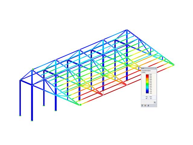
- Graficzne przedstawianie stopni wykorzystania przekroju na wykresie i na modelu w programie RFEM/RSTAB
- Określanie głównych sił wewnętrznych
- Możliwość filtrowania wyników graficznych w programie RFEM/RSTAB
- Graficzne wyświetlanie stopni wykorzystania przekroju i klas przekrojów w renderowanym widoku
- Kolorowe skale w tabelach wyników
- Automatyczna optymalizacja przekrojów
- Transfer zoptymalizowanych przekrojów do programu RFEM/RSTAB
- Wykaz materiałów według prętów i zbiorów prętów
- Bezpośredni eksport danych do aplikacji MS Excel
- Przejrzysty protokół wydruku pozwalający sprawdzić wyniki obliczeń
- W protokole można ująć krzywą temperatury
Podczas obliczania obciążenia rozciągającego, ściskającego, zginającego i ścinającego, moduł porównuje wartości obliczeniowe maksymalnej nośności z wartościami obliczeniowymi oddziaływań.
Jeżeli części są poddane zginaniu i ściskaniu, program dokonuje interakcji. W module RF-/STEEL EC3 można określić współczynniki zgodnie z metodą 1 (załącznik A) lub metodą 2 (załącznik B).
Do obliczeń wyboczenia giętnego nie jest wymagana smukłość ani sprężyste krytyczne obciążenie krytyczne z decydującego przypadku wyboczenia. Moduł automatycznie oblicza wszystkie wymagane współczynniki dla wartości obliczeniowej naprężenia zginającego. Moduł RF-/STEEL EC3 określa sprężysty moment krytyczny dla zwichrzenia dla każdego pręta w każdym miejscu x przekroju. W razie potrzeby wystarczy wprowadzić boczne podpory pośrednie poszczególnych prętów/zbiorów prętów, definiowane w jednym z okien wprowadzania.
W przypadku wyboru prętów do obliczeń odporności ogniowej w module RF-/STEEL EC3 dostępne jest kolejne okno wprowadzania, w którym można wprowadzić dodatkowe parametry, takie jak: typ powłoki lub okładziny. Ustawienia globalne obejmują wymagany czas odporności ogniowej, krzywą temperatury i inne współczynniki. W protokole wydruku wyszczególnione są wszystkie wyniki pośrednie oraz końcowy wynik obliczeń odporności ogniowej. Ponadto w protokole można wydrukować krzywą temperatury.
Wyniki posortowane według przypadku obciążenia, przekroju, pręta, zbioru prętów lub położenia x są wyświetlane w przejrzyście ułożonych oknach wyników. Po wybraniu odpowiedniego wiersza w tabeli wyświetlane są szczegółowe informacje o przeprowadzonych obliczeniach.
Wyniki zawierają zrozumiałą listę wszystkich właściwości materiałów i przekrojów, obliczeniowych sił wewnętrznych i współczynników obliczeniowych. Ponadto w osobnym oknie graficznym można wyświetlić rozkład sił wewnętrznych dla każdego miejsca x.
Szczegółowy i uporządkowany sposób wyświetlania wyników uzupełniają wykazy elementów według prętów/zbiorów prętów dla poszczególnych typów przekrojów. Aby wydrukować dane wejściowe i wyniki, można skorzystać z globalnego protokołu wydruku w programie RFEM/RSTAB.
Wszystkie tabele można eksportować do programu MS Excel w celu dalszego przetwarzania.
Pierwsze okno wyników pokazuje maksymalne stopnie wykorzystania wraz z odpowiednim wykorzystaniem dla każdego obliczanego przypadku obciążenia, kombinacji obciążeń lub kombinacji wyników.
W pozostałych oknach wyników wyświetlane są wszystkie szczegółowe wyniki posortowane według określonego tematu w rozwijanych menu. Wszystkie wyniki pośrednie wzdłuż prętów można wyświetlić w dowolnym miejscu. W ten sposób można łatwo prześledzić, w jaki sposób moduł przeprowadził poszczególne obliczenia.
Pełne dane modułu stanowią część protokołu wydruku programu RFEM/RSTAB. Zawartość i zakres protokołu można wybrać indywidualnie dla poszczególnych obliczeń.
Najpierw należy zdecydować, czy obliczenia mają być przeprowadzone zgodnie z ASD czy LRFD. Następnie można wprowadzić przypadki obciążeń, kombinacje obciążeń i kombinacje wyników, które mają zostać obliczone. Kombinacje obciążeń zgodnie z ASCE 7 można generować ręcznie lub automatycznie w programie RFEM/RSTAB.
W kolejnych krokach można dostosować wstępne ustawienia bocznych podpór pośrednich, długości efektywnych i innych parametrów obliczeniowych specyficznych dla normy, takich jak współczynnik modyfikacjiCb dla zwichrzenia lub współczynnika niezrealizowanego nośności. W przypadku prętów ciągłych można zdefiniować indywidualne warunki podparcia i mimośrody każdego węzła pośredniego pojedynczych prętów. Specjalne narzędzie dla analizy MES, które działa w tle, określa obciążenia krytyczne oraz momenty wymagane dla analizy stateczności.
W połączeniu z programem RFEM/RSTAB, możliwe jest zastosowanie metody analizy bezpośredniej z uwzględnieniem wpływu obliczeń ogólnych zgodnie z teorią drugiego rzędu. W ten sposób unika się stosowania specjalnych współczynników powiększenia.
- Wymiarowanie prętów i zbiorów prętów dla rozciągania, ściskania, zginania, ścinania, kombinacji sił wewnętrznych i skręcania
- Analiza stateczności dla wyboczenia i zwichrzenia
- Automatyczne określanie krytycznych obciążeń wyboczeniowych i krytycznych momentów wyboczeniowych dla ogólnych obciążeń i warunków podparcia za pomocą specjalnego programu MES (analizy wartości własnych) zintegrowanego w module
- Alternatywne obliczenia analityczne krytycznego momentu wyboczeniowego dla sytuacji standardowych
- Możliwość zastosowania oddzielnych podpór bocznych do belek i prętów ciągłych
- Automatyczna klasyfikacja przekrojów (zwarty, niezwarty, smukły)
- Obliczenia w stanie granicznym użytkowalności (ugięcie)
- Optymalizacja przekroju
- Szeroki wybór dostępnych przekrojów, takich jak np. dwuteowniki walcowane; ceowniki; teowniki; kątowniki; profile zamknięte prostokątne i okrągłe; pręty okrągłe; przekroje symetryczne i niesymetryczne, parametryczne przekroje dwuteowe, teowe, kątowniki; podwójne kątowniki
- Przejrzyste okna wprowadzania i wyników
- Szczegółowa dokumentacja wyników wraz z odniesieniami do równań obliczeniowych z zastosowanej normy
- Różne opcje filtrowania i sortowania wyników, w tym listy wyników według prętów, przekrojów i położenia x, przypadków obciążeń, kombinacji obciążeń i kombinacji wyników
- Tabela wyników dla smukłości pręta i głównych sił wewnętrznych
- Wykaz części z parametrami masy i masy
- Pełna integracja z programem RFEM/RSTAB
- Jednostki metryczne i anglosaskie
W obliczeniach nośności przekroju uwzględniane są wszystkie kombinacje sił wewnętrznych.
W przypadku wymiarowania przekrojów metodą MTP, siły wewnętrzne przekroju, działające w układzie osi głównych odniesionych do środka ciężkości lub środka ścinania, są przekształcane na lokalny układ współrzędnych w środku środnika i jest zorientowana w kierunku środnika.
Poszczególne siły wewnętrzne są rozkładane na górną i dolną półkę oraz na środniku, a także określane są graniczne siły wewnętrzne części przekroju. O ile naprężenia tnące i momenty w pasie mogą być przenoszone, nośność osiowa i nośność graniczna na zginanie przekroju są określane za pomocą pozostałych sił wewnętrznych i porównywane z istniejącą siłą i momentem. W przypadku przekroczenia naprężenia ścinającego lub nośności pasa obliczeń nie można przeprowadzić obliczeń.
Metoda Simplex określa zwiększający się współczynnik plastyczny dla zadanej kombinacji sił wewnętrznych na podstawie obliczeń SHAPE-THIN. Odwrotna wartość współczynnika powiększenia stanowi stopień wykorzystania przekroju.
Przekroje eliptyczne są analizowane pod kątem ich nośności plastycznej, korzystając z nieliniowej optymalizacji analitycznej. Metoda ta jest podobna do metody sympleks. Oddzielne przypadki obliczeniowe umożliwiają elastyczną analizę wybranych prętów, zbiorów prętów i oddziaływań oraz poszczególnych przekrojów.
Parametry istotne dla obliczeń, takie jak np. obliczenia wszystkich przekrojów zgodnie z metodą sympleks.
Wyniki obliczeń plastycznych są jak zwykle wyświetlane w RF-/STEEL EC3. Odpowiednie tabele wyników zawierają siły wewnętrzne, klasy przekrojów, obliczenia ogólne i inne dane wynikowe.
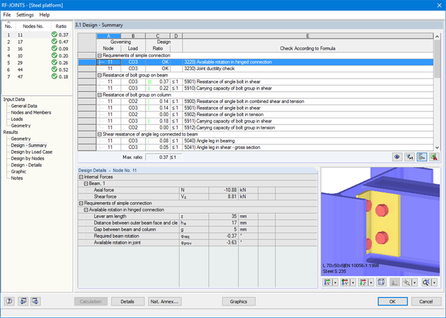
W oknach wyników wyszczególnione są wszystkie wyniki obliczeń. Ponadto tworzone są grafiki 3D, w których poszczególne elementy oraz linie wymiarowe można wyświetlać lub ukrywać. W podsumowaniu można sprawdzić, czy potwierdzono poprawność obliczeń: Stopień wykorzystania jest dodatkowo wizualizowany za pomocą zielonego paska danych, który zmienia kolor na czerwony, gdy obliczenia nie są spełnione. Ponadto wyświetlany jest numer węzła i decydujące PO/KO/KW.
Podczas wyboru obliczeń wyświetlane są szczegółowe wyniki pośrednie wraz z oddziaływaniami i dodatkowymi siłami wewnętrznymi wynikającymi z geometrii połączenia. Istnieje możliwość wyświetlenia wyników według przypadków obciążeń i węzłów. Połączenia są przedstawione w realistycznym renderingu 3D, który można skalować. Oprócz głównych widoków, połączenie można zobaczyć z każdej strony.
Grafiki z wymiarami i opisami można dodać do wydruku programu RFEM/RSTAB lub eksportować jako DXF. Protokół wydruku zawiera wszystkie dane wejściowe i wyniki, przygotowane dla inżynierów testujących. Wszystkie tabele można wyeksportować do programu MS Excel lub do pliku CSV. Wszystkie dane wymagane do eksportu definiuje się w specjalnym menu dla transferu.
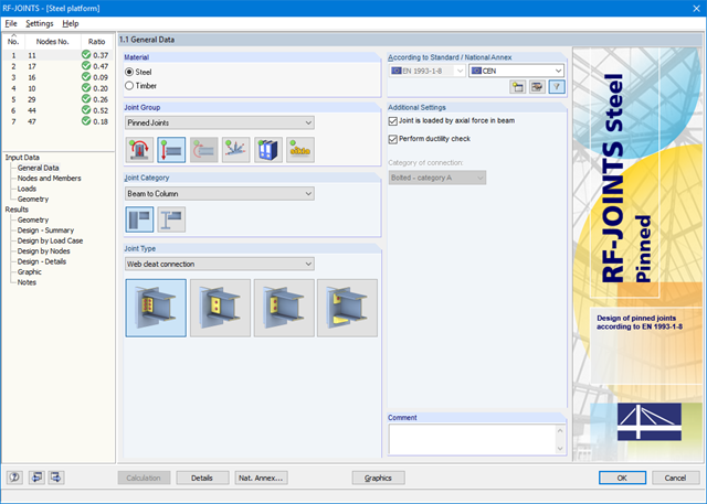
Po otwarciu modułu należy wybrać grupę połączeń (Połączenia przegubowe), następnie kategorię oraz typ połączenia (środnik nakładkowy, blacha zakładkowa, blacha czołowa, blacha czołowa z podkładką). Następnie można wybrać węzły do obliczeń w modelu RFEM/RSTAB. RF-/JOINTS Steel - Pinned automatycznie rozpoznaje pręty połączenia i określa na podstawie ich położenia, czy są to słupy czy belki.
W razie potrzeby można wyłączyć określone pręty z obliczeń. Konstrukcyjnie podobne połączenia można projektować jednocześnie dla kilku węzłów. Obciążenia wymagają wyboru miarodajnych przypadków obciążeń, kombinacji obciążeń lub kombinacji wyników. Alternatywnie można ręcznie wprowadzić przekrój i obciążenie. W ostatnim oknie wprowadzania danych połączenie jest konfigurowane krok po kroku.