AIJ Examples Case E - Building Complex in Actual Urban Area with Dense Concentration of Buildings in Niigata City

Introduction

The Architectural Institute of Japan (AIJ) has presented a number of well-known benchmark scenarios of the wind simulation.
The following article deals with "Case E - Building Complex in Actual Urban Area with Dense Concentration of Low-Rise Buildings in Niigata City".
In the following text, the described scenario is simulated in RWIND 2 and the results are compared with the simulated and experimental results by the AIJ.

Model Layout

Case E describes a realistic city section with predominantly dense development but not very high buildings. Only a few buildings stand significantly above the rest. A more precise description of the geometry or the position of the individual measuring points is irrelevant due to the very complex geometry. The complete geometry was made available by the authors as a CAD file [1] and imported into RFEM for this article in order to be able to transfer it to RWIND.

The model layout is shown below.

01 Model Building from Above - AIJ Case Study: Actual Urban Area with Low-Rise Buildings in Niigata City, Japan

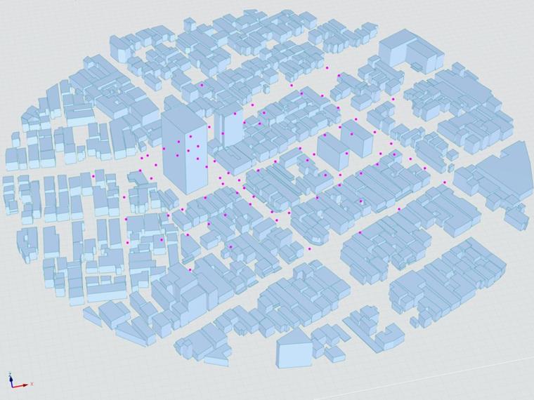
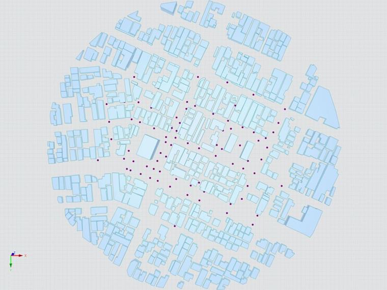
The flow velocity was evaluated in the simulation at clearly defined points. The exact position of the measuring points has also been published [1].

The position of the measuring points is shown below.

02 Model Building from Above - AIJ Case Study: Actual Urban Area with Low-Rise Buildings in Niigata City, Japan

In contrast to models with less geometric complexity, the setting of the level of detail when creating the mesh in RWIND is highly relevant in this case. For a low level of detail, such as default value 2, the shrink-wrapping mesh closes alleys between buildings or inner courtyards. Therefore, we strongly recommend setting the level of detail to the maximum value of 4. The following shows the problem with a mesh density of 15%.

03 Meshing - Level of Detail 2 and Mesh Density of 15%

04 Meshing - Level of Detail 4 and Mesh Density of 15% 

Despite the same setting with regard to the mesh density, there is a considerable difference in the number of elements and thus in the mesh quality. Therefore, we recommend using Level of Detail 4 in all cases and optimizing the mesh density solely on the basis of this setting.

In the AIJ experiment, a corresponding model was set up in a wind tunnel and the wind speed was measured at the mentioned points using split fiber probes.
The authors used three modeling approaches, of which only "Code T" is used in this article. This model was selected because it is an unspecified commercial solver, instead of an individually developed code that would be easier to apply to special purposes, and because RWIND is also a commercial tool.
The comparison of RWIND with all three modeling approaches was omitted for purposes of clarity. Furthermore, the results of the different approaches in the publication [1] do not differ significantly in terms of quality. The comparisons presented here are therefore very similar with the other two models as well.

RWIND Pro 2.02 was used for this article. The model structure in RWIND was adapted as closely as possible to the structure of the reference CFD. The standard k–ε was used as the turbulence model, assuming a steady flow. The comparisons made here relate to the western wind direction in the publication [1]. For the following comparisons of the relative wind speed, it was standardized over 2.77 m/s.

The flow velocity over the height is shown below.

The experimental results of the AIJ were published on their website [1].
The displayed data of the AIJ simulation were determined using the ENGAUGE Digitizer tool [2] from the plots of the publication [1], since the exact values for this were not published.
However, the accuracy of the extracted points should be sufficiently accurate (in the range +-0.5%) and therefore easily comparable.

Another important influencing factor is the "Boundary Layers" setting, which significantly increases the mesh density around the lower boundary condition (soil). In general, the meshing close to the ground influences the results in this region more than would be the case with a greater distance to the ground, because the ground boundary condition has a strong influence. Due to the highly complex geometry of the city, the setting mentioned above was activated and the number of extra layers ("NL") set to 10.

Ergebnisse and Diskussion

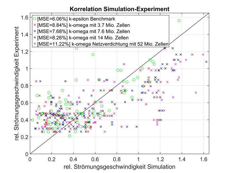
The representation of the three-dimensionally positioned measuring points via simple one-dimensional numbering can be difficult to interpret. Therefore, direct comparisons of the experiment (x-axis) and simulation (y-axis) are shown below for all measuring points. The closer a measuring point is to the diagonal line y=x, the greater the correlation between the simulation and the experiment.

05 Simulation Correlation with Experiment with High Element Number for Different Turbulence Models

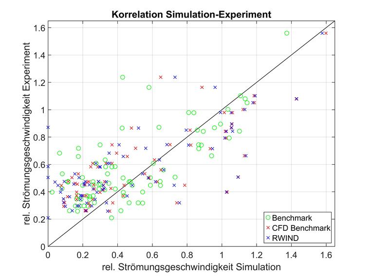
The mean square deviation (MSD) was used as a comparison criterion, but a comparison of the determination coefficients would also show the same behavior, for example. The mean square deviation was preferred to the coefficient of determination because the ratio of experimental and simulated flow velocity does not represent a regression and thus would only be a kind of weighting of individual deviations and not a goodness of fit. The MSD is geometrically easier to interpret with the same expressiveness.

The region near the tallest building stands out in particular; that is, those points with the lowest flow velocity in the experiment. For this group of points, a higher degree of correlation can be observed between RWIND and the experiment than between RWIND and the AIJ simulation. This region will be examined more closely in the later detailed analysis.

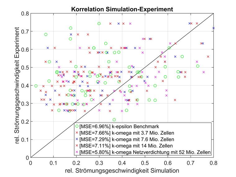
In general, it is advisable to take a closer look at the influence of the mesh density. In the following, meshes of different densities with an otherwise identical model structure and a k-epsilon RAS turbulence model are compared with the literature benchmark. The results are shown below.

06 Simulation Correlation with Experiment Benchmark and RWIND k-Epsilon Simulations with Different Number of Elements

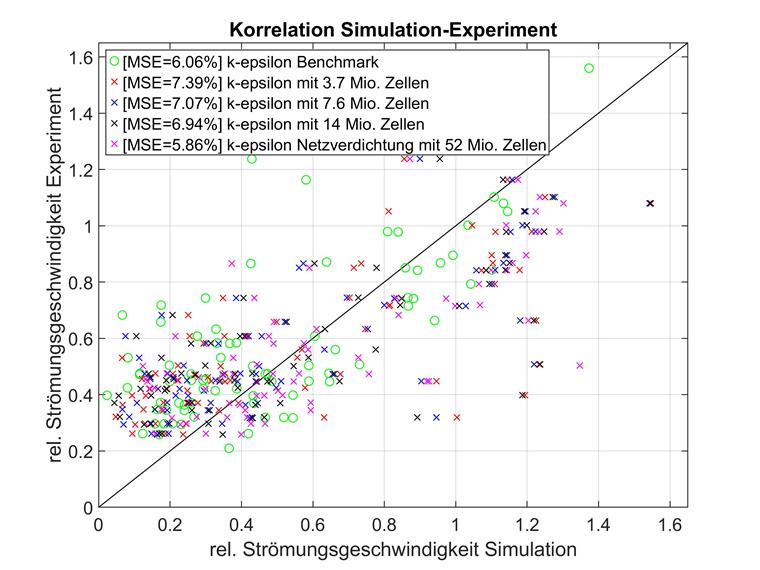
The individual data points lie in the range of the relative flow velocity, especially between 0 and 0.8. The correlation with the experiments sometimes differs significantly within and outside of the stated range. For better comparability, only the data points with rel. flow velocities below 0.8 are shown for both axes and the mean square deviations are recalculated accordingly.

07 Simulation Correlation with Experiment for Rel. Flow Velocities Below 0.8 Benchmark and RWIND k-Epsilon Simulations with Different Number of Elements

A mesh convergence study was also carried out for the k-omega turbulence model and the same mesh formations. The results are shown below.

08 Simulation Correlation with Experiment Benchmark and RWIND k-Omega Simulations with Different Number of Elements

As with the comparison of the k-epsilon models, the low flow velocities were compared separately for k-omega. These data are visualized below.

09 Simulation Correlation with Experiment Flow Velocities Below 0.8 Benchmark and RWIND k-Omega Simulations with Different Number of Elements

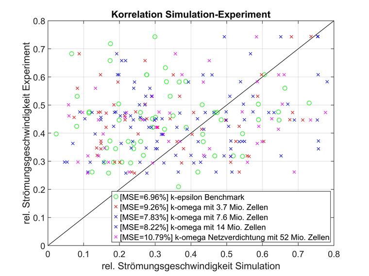
The findings from the comparison of the k-epsilon models are confirmed here. For lower-resolution meshes, the relative flow velocities below 0.8 deviate more from the experimental benchmark than from the mean overall data points.
With an increasing number of elements, however, this effect is reversed, so that closely meshed models deviate even less for the low relative flow velocities.

The points included in this separate consideration tend to be located in more densely built-up areas. The location of the points could explain the better results of the more complex meshes, because the finer meshes can represent the geometry more accurately. Since the real geometry influences these points more than the points with relative flow velocities above 0.8, the denser mesh fits the experiment better.

10 Residuals for Both Turbulence Models - Case E

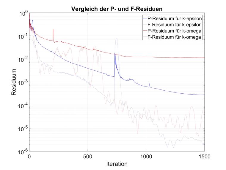
These observations coincide with the expectations of various turbulence models. For the use of k-omega, we thus recommend increasing the number of maximum iterations considerably. The default value of 300 should be increased manually to at least 1,000.

In conclusion, the comparison of both turbulence models in RWIND is less clear for Case E than for Case D, for example. In this reference example, the k-epsilon model is superior for any mesh density. Moreover, k-epsilon scales much better than k-omega as the number of elements increases. The results of the latter turbulence model do not seem to follow any convergence with higher mesh density. The medium complexity model gives the best results, whereas the very complex model shows the greatest deviation by far from the experimental benchmark. Thus, the results of k-epsilon are within the expected range and can also beat the reference simulation if the mesh density is high, but no congruent conclusions can be drawn for k-omega. The very high deviation for the largest k-omega model in particular is a mystery. Presumably, an influencing factor of k-omega, but not equally affecting k-epsilon, could not be conclusively identified.

For a clearer comparison of the reference simulation with the RWIND results, it is advisable to consider the flow velocities as a bottle color image.
The considered section around the tallest building was adapted to that of the authors [1]. The result is shown below.

11 Flow Velocity Around Tallest Building - AIJ Case E

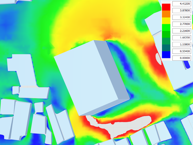
For copyright reasons, the false color images are not compared side by side at this point.

Furthermore, the false color image of the flow velocity over the entire city was shown at the level of the measuring points.

12 Flow Velocity over Entire City - AIJ Case E

There is also very good correlation with the literature simulation. Smaller deviations occur mainly at building corners with a sharp flow, but these are small in terms of amount and are spatially very limited.

Summary

The mean square deviations of different combinations of element number and turbulence model are summarized below.

In the following, there is a comparison of the different speed ranges.

[1] https://www.aij.or.jp/jpn/publish/cfdguide/index_e.htm
[2] https://markummitchell.github.io/engauge-digitizer/