9766x

001660

Stefan Hoffmann, M.Sc.

2020-10-14

Dynamic Analysis of Structures Under Blast Loads

In this article, representations of a blast scenario of a remote detonation performed in RF-DYNAM Pro – Forced Vibrations are shown, and the effects are compared in the linear time history analysis.

1 Representations for Blast Scenario of Remote Detonation in RF-DYNAM Pro – Forced Vibrations

Basics

A structural system must be planned and designed in such a way that it bears up against possible actions and impacts beyond its service life and fulfills the required serviceability. In this regard, actions are classified according to their temporal change as follows:

Permanent actions (for example, self-weight)
Variable actions (for example, live loads, snow, and wind loads)
Exceptional actions (for example, a blast or a vehicle impact)

This technical article deals with the extraordinary action of an explosion. An extraordinary action is of short duration and does not occur with any nameable probability. However, it can have significant consequences on the structure's stability.

"An explosion is a 'suddenly occurring, extremely rapid' oxidation or decomposition reaction with a sudden increase in temperature and pressure. This leads to a sudden volume expansion of gases and the release of large amounts of energy in a small space (…). A sudden volume expansion causes a blast that can be described for an ideal explosion (emanating from a single point source) by a blast wave model." [1] In addition to the air blast loading, an explosion comes with more impact due to high temperatures or projection (splinters, debris). In this article, the loading of a remote detonation is represented as a pure air blast loading on a structure, but no other effects of the explosion.

Air Blast Loading of Remote Detonation

The air blast load can be displayed schematically as a pressure-time curve (from [2]).

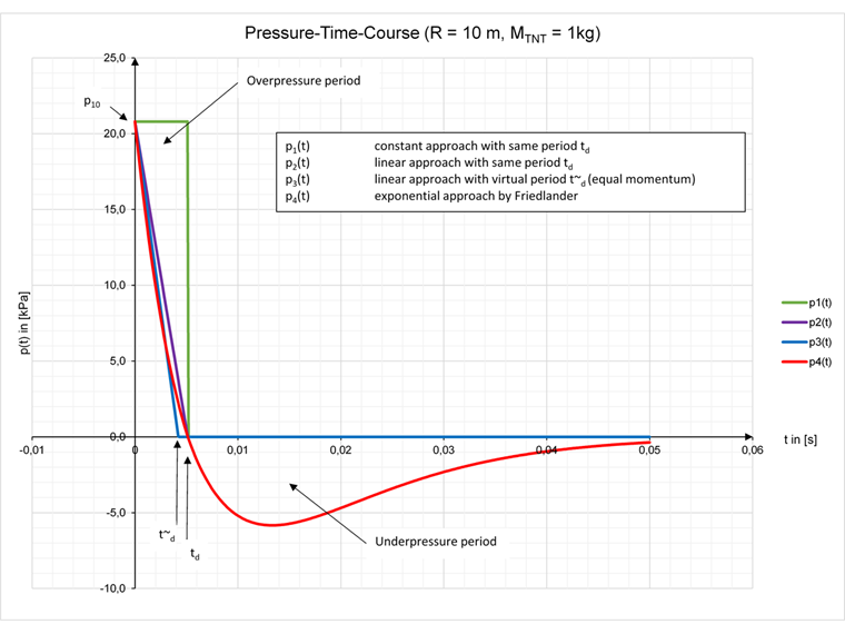
2 Pressure-Time Course of Remote Detonation

The free air shock wave hits the structure abruptly with peak overpressure. The curve includes an overpressure period acting on the structure until the time period t_d is reached, which is reduced by an underpressure period until the ambient air pressure is reached. This exponential approach is often simplified to the overpressure region. In this case, a virtual time t^~_d (t^~_d < t_d) can be calculated that describes the approach linearized with the same amount of momentum, but completely neglects the underpressure period.

The relevant input values for calculating the explosion are the distance to the explosion center R as well as the explosive mass as TNT equivalent M_TNT. The following formulas refer to the load model developed in [2]. A scaled distance Z is determined from both input values, R and M_TNT.

Z = \frac{R}{\sqrt[3]{M_{TNT}}} Z > 0.5 (remote detonation)

Z	Scaled distance [m/kg^1/3] for Z > 2.8
R	Distance to the explosion center [m]
M_TNT	Mass of a TNT equivalent [kg]

Remote Explosion, Scaled Distance

In the following text, the maximum peak overpressure, the positive specific impulse, and the shape coefficient are calculated. The shape factor has a significant influence on the expression of the underpressure period.

{\hat{p}}_{10} = p_{0} \cdot \frac{808 \cdot [1 + {(\frac{Z}{4.5})}^{2}]}{\sqrt{1 + {(\frac{Z}{0.048})}^{2}} \cdot \sqrt{1 + {(\frac{Z}{0.32})}^{2}} \cdot \sqrt{1 + {(\frac{Z}{1.35})}^{2}}}

p₁₀	Maximum peak pressure of remote explosion (Kinney & Graham) [kPa]
p₀	Atmospheric pressure under normal conditions (101.3 [kPa])
Z	Scaled distance [m/kg1/3]

Maximum Peak Overpressure of Remote Explosion (Kinney & Graham)

i^{+} = 2.1 \cdot \frac{R}{Z^{2}}

i⁺	Positive specific impulse [kPa ms]
R	Distance to the explosion center [m]
Z	Scaled distance [m/kg^1/3] for Z > 2.8

Positive Specific Momentum

α = 1.5 \cdot Z^{- 0.38}

α	Shape factor
Z	Scaled distance [m/kg^1/3] for 0.1 < Z < 30

Shape Factor

In the next step, the duration of the positive pressure action t_d as well as the virtual duration of the positive pressure action t^~_d can be calculated.

t_{d} = \frac{i^{+}}{{\hat{p}}_{10}} \cdot (\frac{α^{2}}{α - 1 + e^{- α}})

t_d	Duration of the positive pressure action
i⁺	Positive specific momentum [kPa ms]
p₁₀	Maximum peak overpressure of remote explosion (Kinney & Graham) [kPa]
α	Shape factor
e	Euler's number

Duration of Positive Pressure Action

{\tilde{t}}_{d} = \frac{2 \cdot i^{+}}{{\hat{p}}_{10}}

t^~_d	Virtual duration of the positive pressure action
i⁺	Positive specific momentum [kPa ms]
p₁₀	Maximum peak overpressure of remote explosion (Kinney & Graham) [kPa]

Virtual Duration of Positive Pressure Action (Triangule Calculation)

To determine the reflected pressure-time curve, a reflection factor for the overpressure period c_r and a reflection factor for the underpressure period c^-_r are determined. An infinitely perpendicular reflection face is assumed. For details on the values, see [2].

c_{r} = \frac{8 \cdot {\hat{p}}_{10} + 14 \cdot p_{0}}{{\hat{p}}_{10} + 7 \cdot p_{0}}

c_r	Reflection factor overpressure
p₁₀	Maximum peak overpressure of remote explosion (Kinney & Graham) [kPa]
p₀	Atmospheric pressure under normal conditions (101.3 [kPa])

Reflection Factor Overpressure

c_{r}^{-} = \frac{1.9 \cdot Z - 0.45}{Z}

c_r^-	Reflection factor underpressure
Z	Scaled distance [m/kg^1/3] for Z > 0.5

Reflection Factor Underpressure

Based on all the determined values, the loading in RF -DYNAM Pro – Forced Vibrations can then be represented by means of the loading model for the complete reflected pressure-time curve

p_{r 0} (t) = \{\begin{cases} c_{r} \cdot {\hat{p}}_{10} \cdot φ (t) & t \leq t_{d} \\ c_{r}^{-} \cdot {\hat{p}}_{10} \cdot φ (t) & t > t_{d} \end{cases}

p_r0(t)	Load model for the fully reflected pressure-time diagram
c_r	Reflection factor overpressure
p₁₀	Maximum peak overpressure of remote explosion (Kinney & Graham) [kPa]
φ(t)	Load function (constant/linear/exponential approach)
t_d	Duration of the positive pressure action
c_r^-	Reflection factor underpressure

Load Model for Fully Reflected Pressure-Time Diagram

and any selected loading functions as time diagrams (functions).

p_{1} (t) = \{\begin{cases} {\hat{p}}_{r 0} & t \leq t_{d} \\ 0 & t > t_{d} \end{cases}

p_{2} (t) = \{\begin{cases} {\hat{p}}_{r 0} \cdot (1 - \frac{t}{t_{d}}) & t \leq t_{d} \\ 0 & t > t_{d} \end{cases}

p_{3} (t) = \{\begin{cases} {\hat{p}}_{r 0} \cdot (1 - \frac{t}{{\tilde{t}}_{d}}) & t \leq {\tilde{t}}_{d} \\ 0 & t > {\tilde{t}}_{d} \end{cases}

p_{4} (t) = {\hat{p}}_{r 0} \cdot (1 - \frac{t}{t_{d}}) \cdot e^{- α \cdot \frac{t}{t_{d}}}

p₁(t)	Load function of the constant momentum
p₂(t)	Load function of the linear momentum
p₃(t)	Load function of the linear momentum with the virtual time
p₄(t)	Load function exponential (approach by Friedlander)
t^~_d	Virtual duration of the positive pressure action
t_d	Duration of the positive pressure action
e	Euler's number
α	Shape factor
p_r0	Fully reflected pressure-time diagram

Load Functions

Input in RF -DYNAM Pro – Forced Vibrations

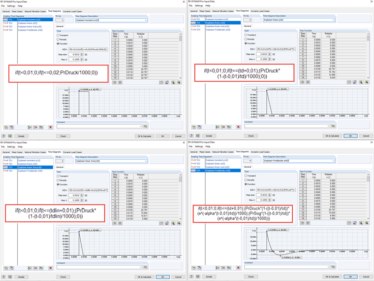
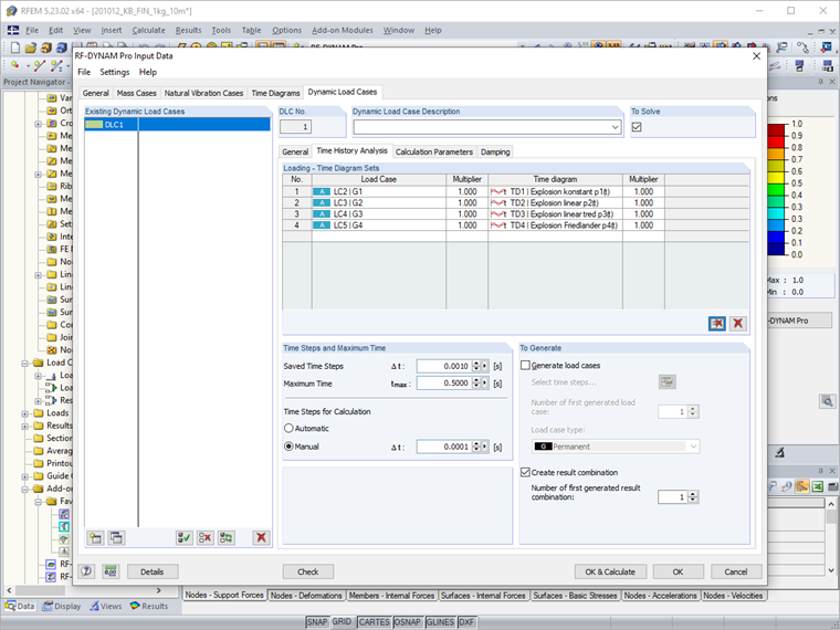
In the add-on module, the loading functions can be entered as time diagrams. Time diagrams can be defined either transiently, periodically, or directly as a function. They excite the structure in a specific position. The position of the load is defined in static load cases. Almost any load type can be entered here. The static load cases are linked to the time diagrams. This happens in the dynamic load cases. The multiplier k is used to determine the final magnitude of the excitation force.

For the following calculations, a remote explosion of M_TNT = 1 kg at a distance of R = 10 m is shown. This results in the following values when using the parameterized input.

3 Parameter List

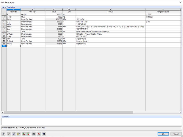
In the parameter list stored in the RFEM model file, only the values for R and M_TNT have to be adjusted. If these are in the value ranges for the scaled distance of 5 < Z < 30, the calculation model presented in [2] can be used.

With the values calculated in the parameter list, the entries for the four displayed time diagrams in the add-on module have been made as follows. As with many numerical programs, the pressure is not applied directly at t = 0 s, but in our example at t = 0.01 s. The use of nested If-functions is useful here to represent the desired functions.

4 Overview: Input of Time Diagrams

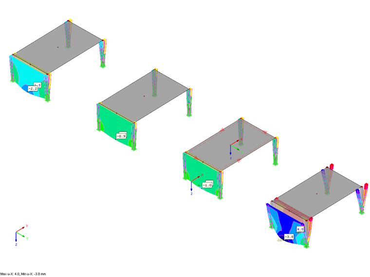
To compare the four functions in one file, four identical subsystems are analyzed in a dynamic load case. A load case is assigned to each subsystem affecting the front surface by 1 kN/m². Moreover, a different time diagram and thus a different load function is assigned to each subsystem.

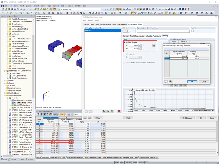
5 Dynamic Load Case: Time Diagram Sets

Finally, the Rayleigh damping of the subsystems is entered, which can be determined from the two dominant mode shapes of the subsystems in the considered direction.

6 Dynamic Load Case: Damping

Results

After calculating and determining the results, you can compare the four loading functions and their effects on the subsystems in the file. This article compares acceleration and displacement in the global X-direction only briefly. You can evaluate the results with the graphical user interface in the Result Navigator. Various result values for the calculated time steps can be displayed here. In addition, after analyzing a dynamic load case, you can access the time history diagram by displaying and comparing the further values of the points. The values in the middle of the front surfaces are considered here.

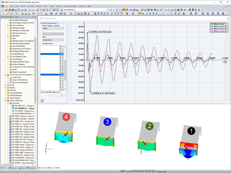
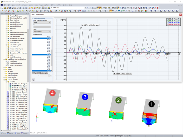
7 Results of Time Course Diagram: Acceleration in Global X-Direction

8 Results of Time Course Diagram: Displacement in Global X-Direction

The application of the constant momentum p₁(t) shows the largest values, as expected. The two linearized curves p₂(t) and p₃(t) are very similar, with the values of p₂(t) > p₃(t) as expected. In the end, the course of p₄(t) shows that considering the underpressure period cannot be neglected and that larger values act on the structure compared to the common, linearized approach of p₃(t).

Conclusion

Representing the real pressure-time curve of a remote detonation by means of time diagrams in RF-DYNAM Pro – Forced Vibrations is an effective way to determine the effects of the over- and underpressure periods on the structure. The model's parametrization allows you to represent and compare different blast scenarios by adjusting R and M_TNT.

Knowledge Base

KB 001660 | Dynamic Analysis of Structures Under Blast Loads

Author

Mr. Hoffmann is responsible for development in the areas of dynamic analysis, membrane structures, and RWIND. Furthermore, he provides technical support for our customers.

Links

Dynamic and Seismic Analysis

References

;