


ASCE 7-22 and P-Delta Effects
ASCE 7-22 Standard [1], Sect. 12.9.1.6 further refers to Sect. 12.8.7 [1], which states that P-delta does not need to be considered when the stability coefficient (θ) determined by the equation below is equal to or less than 0.10.
|
Px |
Total vertical design load at and above level x per Sect. 12.8.6.1 (all load factors equal to or less than 1.0) |
|
Vx/Δse |
Story stiffness at level x, calculated as the seismic design shear, Vx, divided by the corresponding elastic story drift, Δe |
|
hsx |
Story height below level x |
The standard continues to state that θ should not exceed the lesser of θmax, given by the equation below, as the structure is potentially unsafe and should be redesigned.
|
Cd |
Deflection amplification factor in Table 12.2-1 |
|
β |
Ratio of shear demand to design shear capacity for the story between levels x and x-1 (taken conservatively as 1.0, but not less than 1.25/Ω0) |
When 0.10 < θ ≤ θmax, it is permitted for displacements and member forces should be multiplied by a factor of 1.0/(1-θ). Alternatively, P-delta effects can be included in an automated analysis, where θmax limitations are still applicable.
NBC 2020 and P-Delta Effects
In Sent. 4.1.8.3.8.c of the NBC 2020 [2], only a short requirement is given that sway effects due to the interaction of gravity loads with the deformed structure should be considered. However, the NBC 2015 Commentary [3] gives further explanation similar to the ASCE 7 standard where the stability factor (θx) at level x should be calculated with the given equation below.
|
\[ \sum_{i=x}^{n} W_i \] |
Portion of the factored dead plus live load at level x |
|
\[ \sum_{i=x}^{n} F_i \] |
Sum of the design lateral seismic forces acting at or above level x |
|
Ro |
Overstrength-related modification factor |
|
Δmx |
Max inelastic interstory deflection |
|
hs |
Interstory height |
When θx is less than 0.10, then P-delta effects can be ignored. When θx is greater than 0.40, the structure should be redesigned as it’s considered unsafe during extreme earthquakes. For 0.10 ≤ θx ≤ 0.40, the seismic-induced forces and moments can be multiplied by an amplification factor of (1+θx) to account for P-delta. This amplification factor does not need to be applied to displacements.
Approximate Consideration of P-Delta Effects with Amplification Factors
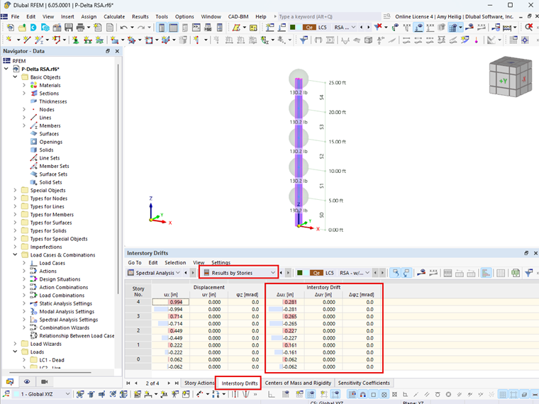
The stability factor value should be calculated in both orthogonal horizontal directions to determine if P-delta is a concern. The required story drift, Δ, necessary to calculate the stability coefficient in both the ASCE 7-22 and NBC 2020, is now given automatically in RFEM 6 with the Building Design add-on. Each story level will include the relevant story drift in table result output as shown in Image 01.
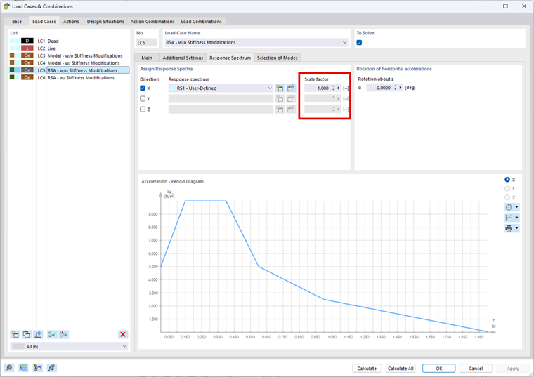
If one or both directions require second-order effects to be considered within the given ranges, the factor 1.0/(1-θ) from the ASCE 7-22 or (1+θx) from the NBC 2020 can easily be accounted for in RFEM 6 and the Response Spectrum Analysis add-on. All resulting forces and/or deflections will be amplified by the set value.
More Exact Consideration of P-Delta Effects with the Geometric Stiffness Matrix
Although secondary effects can be estimated with the amplification factors above, this is a more conservative approach. For scenarios where large story drifts occur or P-delta effects need to be calculated with a more exact approach, the influence of axial forces can be activated in the Response Spectrum Analysis add-on.
When running a dynamic analysis, the typical nonlinear iterative calculations for second-order effects when considering a static analysis are no longer applicable. The problem must be linearized, which is carried out by activating the geometric stiffness matrix during the analysis. With this approach, it is assumed that vertical loads do not change due to horizontal effects and that deformations are small when compared to the overall dimensions of the structure [2].
The concept behind the geometric stiffness matrix is the stress stiffening effect. Tensile axial forces will lead to an increased bending stiffness of a member while compressive axial forces will lead to a reduced bending stiffness. This can be easily conveyed with the example of a cable or slender rod. When the member experiences a tension force, the bending stiffness is significantly greater than when the member is undergoing a compression force. In the case of compression, the member has very little if any bending stiffness to withstand an applied lateral load.
The geometric stiffness matrix Kg can be derived from the static equilibrium conditions.
For simplification, only the degrees of freedom of the horizontal displacement are displayed. The derivation shown is based on the overturning moment approach due to the linear displacement application. This is a simplification for the bending element and an accurate assumption for the truss element. Notice how the matrix is only dependent on the element length and axial force.
More precise determination of the geometric stiffness matrix for bending beams can be obtained by using the cubic displacement approach or the analytical solution of the differential equation of the bending line. More information on theory and derivations are provided by Werkle [4].
The geometric stiffness matrix Kg is added to the system stiffness matrix K, and thus the modified stiffness matrix Kmod is obtained:
Kmod = K + Kg
In the case of compression normal forces, this consequently leads to stiffness reduction.
P-Delta Geometric Stiffness Modification Example in RFEM 6
The application of stiffness reduction utilizing the geometric stiffness matrix to consider second-order effects (P-Delta) in a response spectrum analysis is carried out with a simple cantilever structure in RFEM 6. The member is a W 12x26 cross-section and A992 material with Iy = 204 in4 and E = 29000 ksi. Each of the (5) story height levels are 5 ft for a total height of 25 ft.
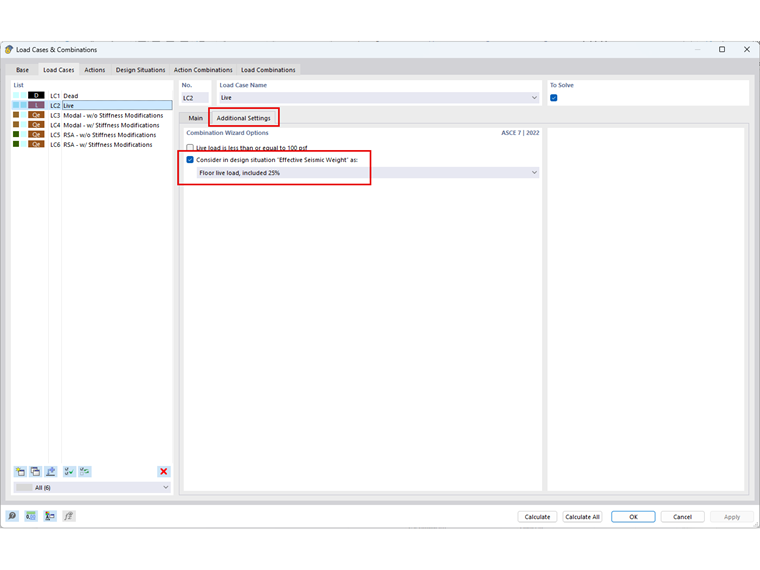
Neglecting self-weight, a 1.5 kip dead load is applied at each level under LC 1: Dead as well as a 3 kip live load at each level under LC2: Live. The Additional Settings under LC2 are activated to consider 25% of the live load automatically for the mass combination.
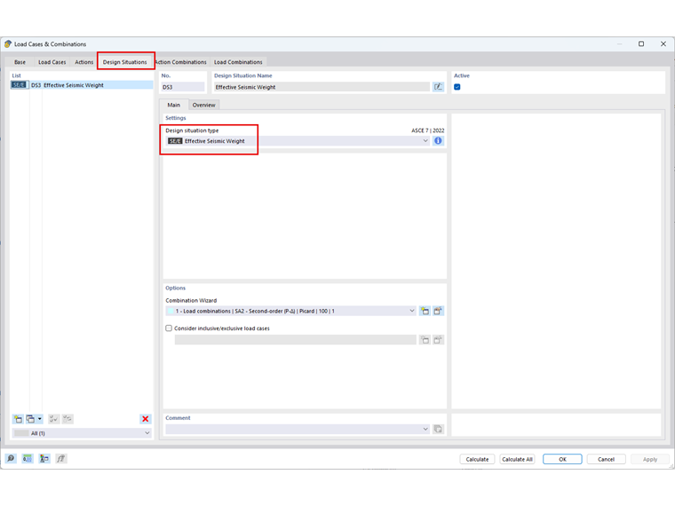
The Design Situation DS1: Effective Seismic Weight is defined to automatically create the mass combination CO1: D + 0.25L. After the mass conversion, a total of 2250.3 lbs at each level are considered in the X-direction for further seismic analysis.
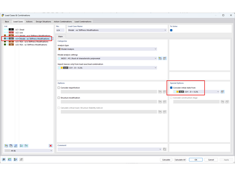
The Modal Analysis add-on will calculate the mode shapes and effective modal masses of a structure. It’s possible to consider an initial state, which will apply a stiffness modification based on defined load cases and load combinations. Two modal analysis load cases are defined. The first is LC3: Modal – w/o Stiffness Modifications to carry out the modal analysis without any stiffness modifications.
For LC4: Modal – w/ Stiffness Modifications, the consider initial state option is activated. The load case or load combination imported here should consider the highest compression axial loads on the structure. For this example, the mass combination CO1 is used to approximate second-order effects with the geometric stiffness modifications.
The following table shows the calculated natural frequencies (f) [Hz] and natural periods (T) [sec] with and without the geometric stiffness matrix Kg considered.
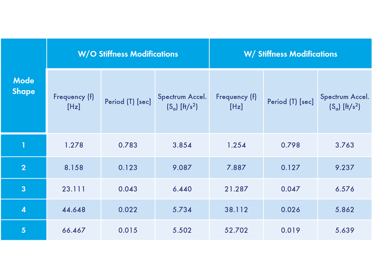
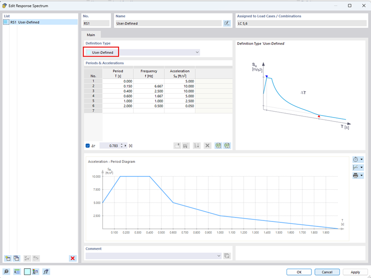
The multi-modal response spectrum analysis refers to the structure’s natural frequencies to determine the acceleration values from the defined response spectrum. Based on these acceleration values, the program determines the response spectrum internal forces. A user‑defined response spectrum is defined for this example, shown below. The acceleration values Sa [ft/s2] determined from the user-defined response spectrum for each eigenvalue are listed in the table above.
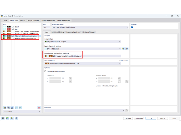
To ensure the correct assignment of the modified frequencies, the desired modal analysis must be selected when defining a response spectrum load case. This means, if the response spectrum analysis should consider the geometric stiffness modifications, the relevant modal analysis with the previously defined stiffness modifications should be referenced.
When applying compression axial forces, the consideration of the geometric stiffness matrix leads to lower natural frequencies of the structure. This can cause lower acceleration values Sa, as seen in this example. Modification of the natural frequencies alone is not enough to consider the second-order theory. In fact, this may lead to smaller results, which can be incorrect. Therefore, it’s important to also use the modified stiffness matrix when calculating the structure’s internal forces and deformations. In the RFEM response spectrum analysis, the modified stiffness from the modal analysis is automatically used for determining the results of the response spectrum analysis when selected. The deformations, internal forces, and support reactions determined in the response spectrum analysis, with and without the geometric stiffness matrix, are shown in Image 08.
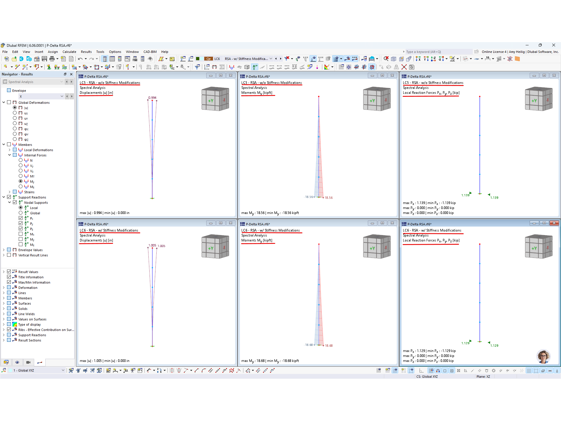_and_with_Stiffness_Modification_(bottom).png?mw=760&hash=a0656d7f5afcb25e57fe07073895766288787ecd)
The consideration of the geometric stiffness matrix leads to larger deformations and internal forces. However, the resulting support loads are slightly smaller when considering the geometric stiffness matrix.
