Determining the Material Properties of Steel-Fiber-Reinforced Concrete and Their Application in RFEM

Material Properties

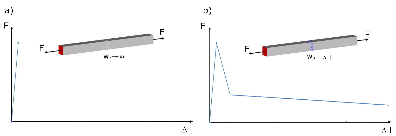
According to DIN EN 206-1, fiber-reinforced concrete is concrete to which steel fiber is added to achieve certain properties. By adding sufficient steel fibers, they can transfer tensile forces across a crack in the concrete. Figure 01 compares the general behavior of unreinforced concrete and steel-fiber-reinforced concrete under tension. You can see that the tension resistance of the steel-fiber-reinforced concrete decreases with increasing deformation, and the load-deformation curve shows a descending branch after the tensile strength is reached.

Load-Deformation Behavior of a) Unreinforced Concrete and b) Steel Fiber-Reinforced Concrete

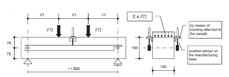
The strength of the steel-fiber-reinforced concrete composite material after exceeding the concrete tensile strength is called post-cracking tensile strength. The tensile forces actually occurring in the steel fibers are related to the surface of the tension zone of the concrete. The post-cracking tensile strength is usually determined by means of a bending tension test according to [1] in the building material laboratory. Beams with the dimensions b/h/l = 150 mm / 150 mm / 700 mm are used as test specimens. Since the bending tension behavior in the post-cracking region is important for the work line of steel-fiber-reinforced concrete, the 4-point bending test is carried out in a displacement-controlled manner. Figure 02 shows the dimensioned graphical representation of the 4-point bending test.

Testing Device to Determine Post-Cracking Flexural Tensile Strength (Dimensions in mm)

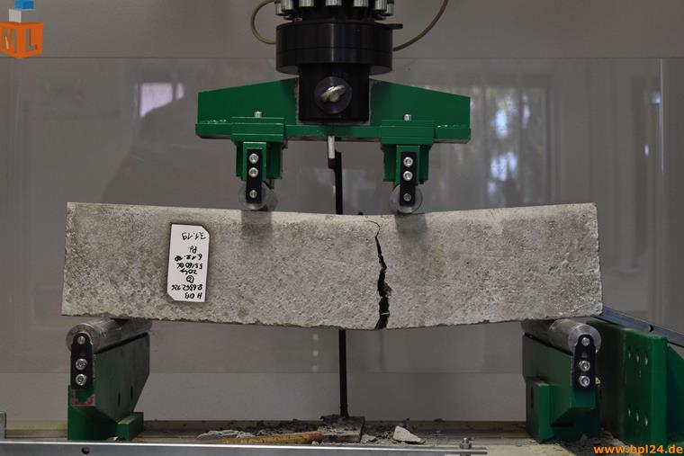
Due to the experimental setup of the 4-point bending test, the position of the crack is arbitrarily on the test beam, because the local loading between the two load points is constant. In the figure below, you can see from the final test (the press was extended manually to increase the crack opening after the end of the test) that the crack formation occurs arbitrarily between the two press rolls at the governing location (= weakest position).

Completed 4-Point Bending Test with Crack Opening (Image: BPL Müller and Lobisch GmbH)

The test results are documented in a load-deformation curve (see Figure 04). The equivalent tensile strengths and, with the help of conversion factors, the post-cracking tensile strength of the steel-fiber-reinforced concrete, are determined from this load-deformation curve. A distinction is made between a characteristic value for the evaluation of the serviceability limit state (= small deformations, δ = 0.5 mm) and a governing parameter for the ultimate limit state (= large deformations, δ = 3.5 mm).

Symbolic Load-Deformation Curve to Determine Post-Cracking Tensile Strengths

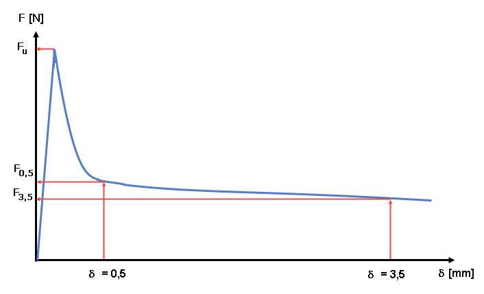
The post-cracking flexural tensile strengths of the steel-fiber-reinforced concrete are to be determined from the load values F_0.5 for δ = 0.5 mm and F_3.5 for δ = 3.5 mm. In this case, the reached load L_i (with i=0.5 and accordingly 3.5) is multiplied by the related load lever arm and divided by the section modulus W_j of the uncracked cross-section. The mean post-cracking flexural tensile strength f^f_cflm,Li of a test series of n test beams is obtained as the arithmetic mean of the individual post-crack tensile strengths.

For classifying the steel-fiber-reinforced concrete composite material, the Steel-Fiber-Reinforced Concrete Guideline of the German Committee for Reinforced Concrete (DAfStb) specifies two different performance classes: L1 and L2. Performance class L1 describes the material properties for small deformations (δ = 0.5 mm) and performance class L2, the behavior for larger deformations (δ = 3.5 mm). The description of the performance classes Li corresponds to the characteristic value of the post-cracking flexural tensile strength f^f_cflk,Li in N/mm² for the corresponding deformations. According to [1], the characteristic post-cracking flexural tensile strength is calculated from the mean post-crack flexural tensile strength f^f_cflm,Li.

where
Lf^f_cflm,Li ... mean value of the logarithmized single test results f^f_cfl,Li,j (for details, see [1])
L_s ... standard deviation of the logarithmized single test results (for details, see [1])
k_s ... fractile correction factor for unknown standard deviations for the 5% fractile with 75% confidence level (for details, see [1])

Thus, the description of the steel-fiber-reinforced concrete is carried out by adding the letter L for the performance class with the characteristic post-cracking flexural tensile strength for the deformations 1 (SLS) and 2 (ULS). For example, steel-fiber-reinforced concrete C30/37 L0.9/L0.6 XC1 has a characteristic post-cracking flexural tensile strength of 0.9 N/mm² for the deformation 1 and 0.6 N/mm² for the deformation 2.

Stress-Strain Curve of Steel-Fiber-Reinforced Concrete

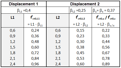
Stress-strain curves are required for the design of structural steel components. For this purpose, the characteristic post-crack flexural tensile strengths f^f_cflk,Li described above are converted into the axial post-cracking tensile strengths f^f_ct0,i by means of β factors according to [1]. Table R3 of the German Committee for Reinforced Concrete (DAfStb) Guideline on steel-fiber-reinforced concrete [1] shows the basic values of the axial post-cracking tensile strength f^f_ct0,i for the respective performance classes (see Figure 05).

Most Common Performance Classes L1 and L2 with Corresponding Basic Values of Axial Post-Cracking Tensile Strength

In order to obtain the calculation values f^f_ctR,i for the stress-strain curve, we have to modify the basic values of the axial post-cracking tensile strength by two correction factors, κ^f_G and κ^f_F .

f^f_ctR,i = κ^f_G ⋅ κ^f_F ⋅ f^f_ct0,i

where
κ^f_G ... factor for considering the influence of the structural component size on the variation coefficient = 1.0 + A^f_ct ⋅ 0.5 < 1.70
A_ct ... the cross-section area subjected to tensile stress of the cracked areas in m² belonging to the respective state of equilibrium
κ^f_F ... factor for considering the fiber orientation = 0.5. For planar, horizontally produced laminar structural components (b <5), an assumption of κ^f_F = 1.0 for bending and tensile stress is allowed.

The Steel Fiber Directive [1] assumes that deformation 1 with δ = 0.5 mm of the 4-point bending test corresponds to a strain of ε = 0.0035, and deformation 2 with δ = 3.5 mm corresponds to a strain of ε = 0.025.

Depending on the provided calculation, different stress-strain curves are available in [1] for the tension area. For a nonlinear determination of deformation and internal forces, the multilinear relation shown in Figure 06 is applied in the tension area. The linear distribution can be applied until the concrete tensile strength f_ctm is reached. According to [1], the stress-strain curve shown in blue in Figure 06 is only allowed for steel-fiber-reinforced concrete with a ratio of L2 / L1 ≥ 0.7. For performance class ratios L2 / L1 ≤ 0.7, only the stress distribution (dotted green line in Figure 06) is allowed to be applied.

Stress-Strain Curve in Tension Area According to [1] to Determine Internal Forces and Deformations in Nonlinear Methods

Application of the concrete tensile strength f_ctm is not allowed for the cross-section design in the ultimate limit state. The additional tensile strength that can be applied comes only from the tensile force in the crack transmitted by the steel fibers. Furthermore, the tensile strengths for the ultimate limit state design with the design values f^f_ctd,Li have to be applied. They are obtained by multiplying the calculated values f^f_ctR,Li by the reduction factor α^f_c and dividing by the partial safety factor γ^f_ct. The application of f^f_ctd,L1 and f^f_ctd,L2 (solid blue line in Figure 7) is restricted to the ratios of L2 / L1 ≥ 0.7. The stress distribution, shown in green with dashes in Figure 07, may be used in a simplified way for ratios L2 / L1 ≤ 1.

Stress-Strain Curve on Tension Side According to [1] for Cross-Section Design in Ultimate Limit State

In the compression zone of the stress-strain curve for steel-fiber-reinforced concrete, there is no difference between normal concrete without fibers and steel-fiber-reinforced concrete. The regulation of EN 1992-1-1 [4] applies unchanged to the stress-strain relation in the compression area. Therefore, a parabolic diagram according to Chapter 3.1.5 [4] (see Figure 08 a) or a parabola rectangle according to Chapter 3.1.6 [4] for the stress-strain curve is used for the nonlinear calculation of the friction and internal forces to be used in the compression area.

Stress-Strain Diagram According to [4] for Compression Zone: a) for Nonlinear Calculation; b) for Cross-Section Design

Nonlinear Calculation with RFEM

According to [1], nonlinear methods may, in principle, be used for structural components of steel-fiber-reinforced concrete if the predominant load-bearing capacity is achieved by reinforcing steel. In all other cases, the nonlinear calculation is only applicable for structural components with elastic foundations, anchored underwater concrete slabs, pile-supported floor slabs, shell-shaped structural components, and monolithic manufactured precast vessels.

In the following text, the stress-strain curve for steel-fiber-reinforced concrete will be defined in RFEM and the material behavior will be checked. For the purposes of this article, this will initially only be carried out on an FE element with a uniaxial tension load. By means of this simple test, the material model used in RFEM is to be verified for the absorption of a uniaxial tension load.

For a nonlinear calculation of internal forces and deformations of steel-fiber-reinforced concrete, the stress-strain curve applied in the compression area consists of a parabola according to 3.1.5 EN 1992-1-1 [4] and in the tension area of the multilinear distribution with consideration of the concrete tensile strength f_ctm (Figure 06). In RFEM, you have to use a material model that can represent the descending branch after the crack formation. With the RF-MAT NL add-on module, RFEM can represent exactly this behavior using the "Isotropic Damage 2D/3D" material model. The "Isotropic Damage" material model was described in detail in an earlier article. 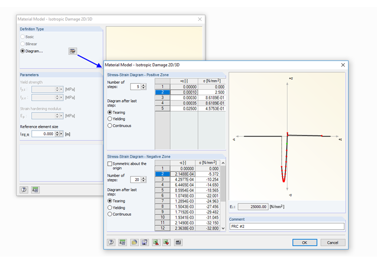The stress-strain curve is generally entered in RFEM. The compression and tension areas can be defined individually using the "Diagram ..." option. Only the elastic modulus at the origin must be identical to the respective subsequent points in the compression and tension areas. The reference element size l_FE,R is left unchanged, with a length of 0.0 m. Thus, it is ensured that the defined stress-strain curve is applied 1:1 in the damage zone in the calculation. Figure 09 shows the input of the analyzed steel-fiber-reinforced concrete in the input window of RFEM.

Defining Stress-Strain Curve of Steel Fiber-Reinforced Concrete

Since the illustration of the post-cracking tension behavior is to be analyzed in detail below, the properties in the tension area of the tested steel-fiber-reinforced concrete are described in detail below:

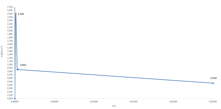
f_ctm = 2.500 N/mm²
1.04 ⋅ f^f_ctr,L1 = 0.862 N/mm²
1.04 ⋅ f^f_ctr,L2 = 0.458 N/mm²

The stress-strain curve shown in Figure 10 results from the aforementioned material parameters for the tension area.

Calculation Model in RFEM: One FE Element, Held on Left, Pulled on Right

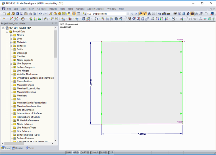
In order to avoid the influence of neighboring elements and biaxial stress states on the results, the material is checked on a finite element with side lengths of 1 ⋅ 1 m. The element is held horizontally on one side of the element, then pulled on the opposite side. To obtain the image of the post-cracking tensile strength, it is necessary to apply the displacement in a time-controlled manner, as in the 4-point bending test described above. Figure 11 shows the calculation model in RFEM.

Defining Incrementally Increasing Loading

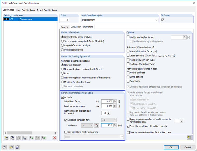
Using the "Incrementally Increasing Loading" option in the calculation parameters of the load case, the deformation is increased until the break-off criterion is reached. The break-off criterion used was defined with a nodal displacement of 25.1 mm, which corresponds to a strain ε of 0.0251.

Displaying First Membrane Stress in Calculation Diagram

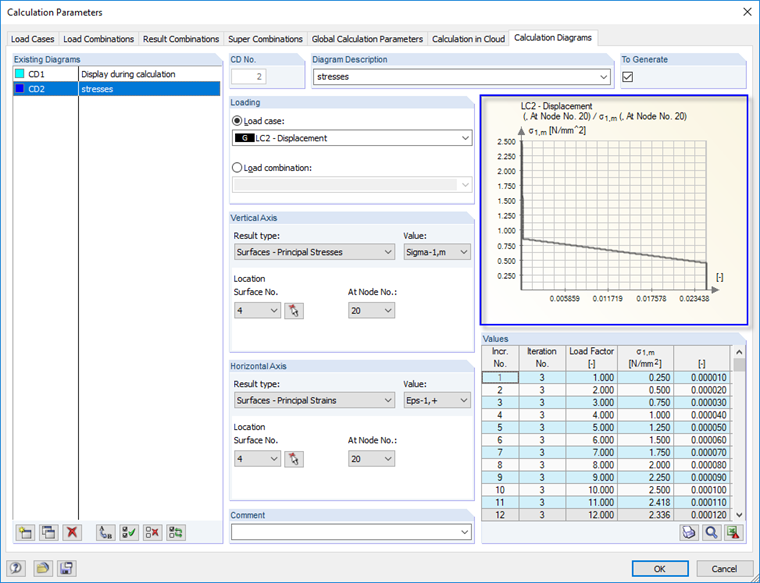
The diaphragm stress in the direction of the principal axis σ_1,m is used to evaluate the results of the calculation. In the "Calculation Parameters" dialog box, you can display a diagram for the calculation results for a step-by-step load increment.

Comparing RFEM Results with Defined Material Property in Tension Area

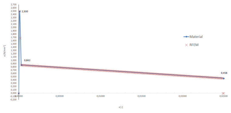
The calculated membrane stress follows the specified distribution of the post-cracking tensile strength exactly. In the following diagram, the main stress ma σ_1,m is defined by the stress-strain curve of the steel-fiber-reinforced concrete defined in the tension area. The results calculated in RFEM match the defined workline precisely.

Stress-Strain Curve of Steel Fiber-Reinforced Concrete in Tension Area for Nonlinear Calculation

Summary

By using the "Isotropic Damage 2D/3D" material model, it was possible to verify precisely the check behavior of the steel-fiber-reinforced concrete in case of uniaxial tension loading. Please note that for such verification calculations, all influences from, for example, neighboring elements, multiaxial stress states, or modification options in the material model, are excluded by specifying a reference element size l_FE,R.