Wind Loads on High Building

The RWIND Simulation program is primarily designed to quickly calculate results even for relatively complex and large models. Default settings were used for a quick calculation, which subsequently took only 5 minutes on a standard PC. The results obtained are in relatively close agreement with those published in the above article [1], and are discussed in more detail below.

Computational Domain and Mesh

The CAARC building is a rectangular prismatic shape with dimensions of 150 ft by 100 ft by 600 ft in height. The wind tunnel dimensions are 4,950 ft in the streamwise direction, 3,000 ft in the spanwise direction, and the total height is equal to 1,200 ft.

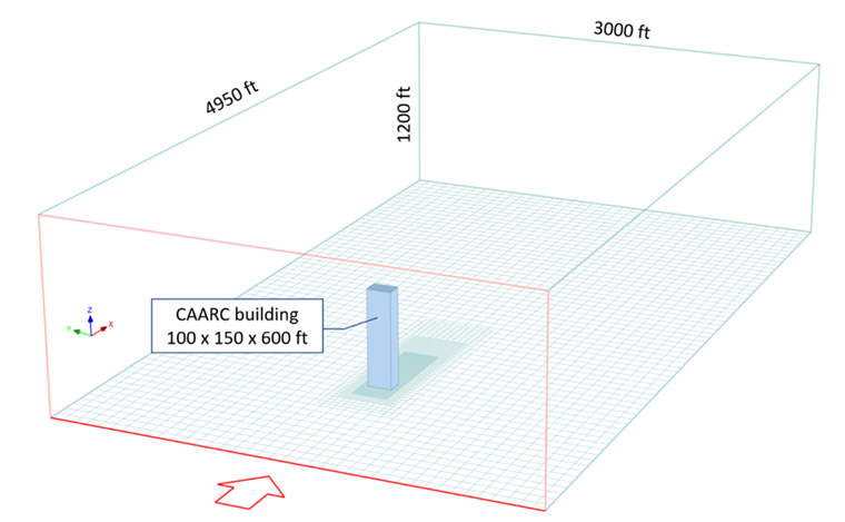
The finite volume mesh was locally refined near the building model with the total number of mesh cells at 540,180. Although RWIND Simulation allows calculations on significantly finer meshes (up to 50 million cells), a relatively coarse mesh was selected for a quick calculation.

Simulation Setup

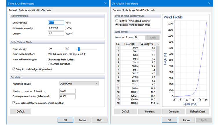
The simulation parameters and the inlet wind velocity profile are defined according to Dagnew et al. [1], and are displayed in Image 02.

The model boundary conditions are described in Table 1.

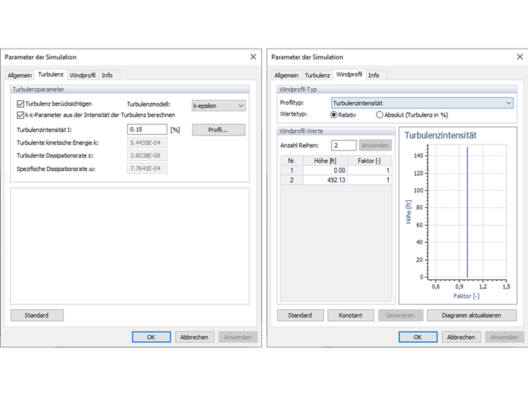
The k‑epsilon turbulence model was used, and the inlet turbulent intensity was set to 0.15%.

Stationary calculation

The calculation was performed with the RWIND Simulation Solver, which is relative to the OpenFOAM-SIMPLE family of solvers. It is a steady-state solver for incompressible, turbulent flow. The entire simulation, including mesh generation and result preparation, was completed in 5 minutes on a PC with 8 cores (Intel i9‑9900K). The residual pressure convergence criterion was set to 0.001, which is the standard value for the quickest calculation, and was achieved after 350 iterations. The minimum residual pressure is 0.0001, and it could be reached after 700 iterations while continuing the calculation. However, the results were not significantly affected.

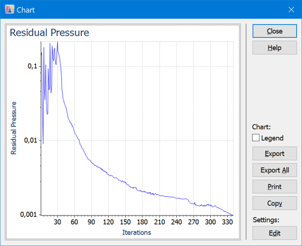
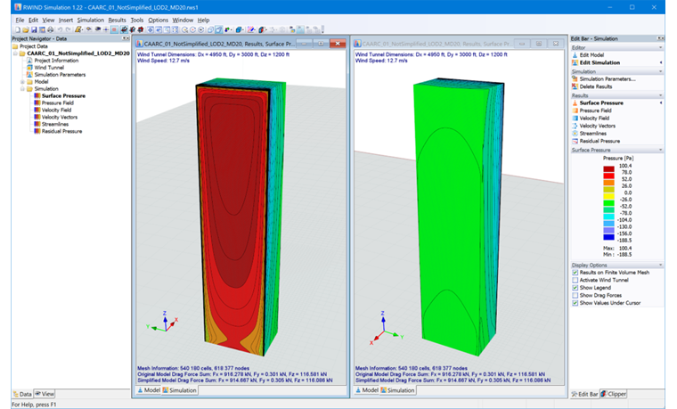
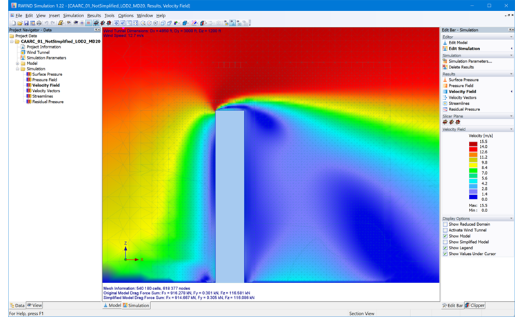
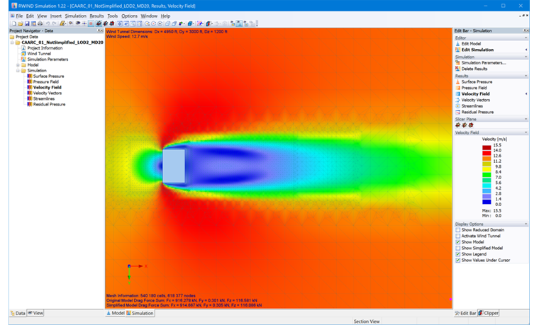
Image 05 through Image 07 show the pressure distribution on the building surface and the velocity field. For validation and comparison purposes, the calculated pressure coefficient c_p is compared to the data obtained from [1] in Image 9 through Image 11. The c_p coefficient is calculated as follows:

Pressure coefficient

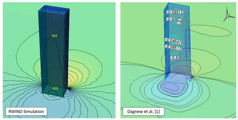
The RWIND Simulation results and experimental results according to Dagnew et al. [1] on the windward face are in close comparison. On the sidewall and leeward faces, 10% - 20% differences between the measured and the calculated data are observed, which can be explained by the turbulence model (k-epsilon) used and the coarse computational mesh. The result accuracy can be improved by using more accurate turbulence models (LES), which will be available in future versions of RWIND Simulation.

RWIND Simulation Results:

Comparison with the data and results published in [1]:

To explain the previous diagram, it can be added that the unit of the abscissa axis x '/Dx results from the actually existing x coordinate from RWIND and the center distance from RWIND, which is 100 ft.

Transient calculation

For tall and slender structures, it is useful to simulate a transient (unsteady) flow in order to consider possible damage caused by vortex shedding. RWIND 2 uses the “BlueDySolver” for simulating unsteady flows, which was developed from the standard OpenFOAM® solver “PimpleFoam”. As part of this simulation, 91 flow animations were created over a simulation time of 1200 seconds with a time step of 12 seconds. The program offers the possibility to change these time slices automatically and to smooth the flow between two time slices by linear interpolation in such a way that a coherent animation of the flow can be displayed over the entire simulation time. The following animations show the pressure distribution on the building surface as well as the velocity distribution around the building, which were achieved with the help of the transient calculation.

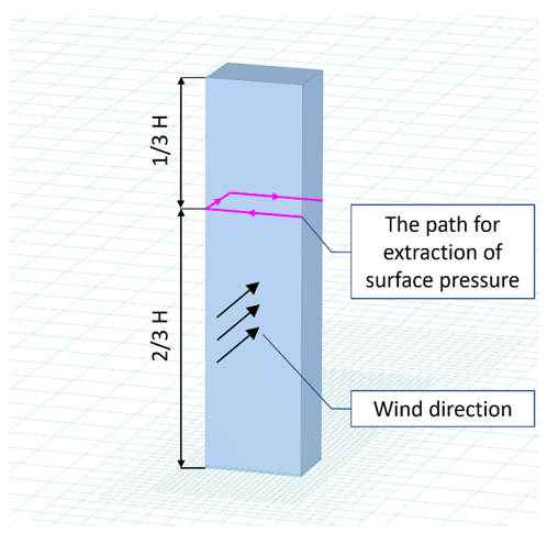
To compare the results of the transient calculation with those of the stationary calculation or those of Dagnew et al. [1] , the pressure coefficient c_p for the evaluation path shown in Figure 08 was also determined for this simulation. The following diagram shows all of the results.

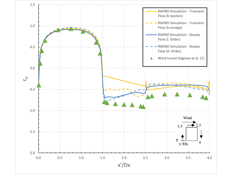
The results of the transient calculation on the windward surface also agree very well with the results of the stationary calculation and the experimental wind tunnel test data by Dagnew et al. [1] . At the leeward surface, the results of the transient flow, similar to those of the steady flow, deviate by approx. 10 to 20% from the measured data. The deviations of the transient results from the other results are slightly larger on the side surfaces. On the one hand, this can be attributed to the fact that the RWIND Simulation software uses a different solver for the transient calculation than for the stationary simulation and, on the other hand, to the continuous further development and improvement of the software. This comparison also shows that the K-Omega turbulence model provides greater agreement with the experimental results than the K-Epsilon turbulence model. In addition, the stationary simulation has been expanded to include a second-order calculation. These results are also shown in the previous diagram, but differ only slightly from those according to the first order.