4.3 Materials

Materials are required to define surfaces, cross-sections, and solids. The material properties affect the stiffnesses of these objects.

A Color is assigned to each material, which is used for the display of objects in the rendered model (see Chapter 11.1.9).

For new models, RFEM presets the two materials that were last used.

Any name can be chosen as a Description of the material. When the entered name corresponds to an entry of the library, RFEM imports the material properties.

The modulus of elasticity E describes the ratio between normal stress and strain.

To adjust the settings for Materials, click Edit → Units and Decimal Places on the menu or use the corresponding button.

The shear modulus G is the second parameter for describing the elastic behavior of a linear, isotropic, and homogenous material.

The following relation exists between modulus E and G, as well as Poisson's ratio ν:

$E=2G \left(1+\nu \right)$

Generally, Poisson's ratio of isotropic materials is between 0.0 and 0.5. Therefore, for a value of 0.5 or higher (e.g. rubber), we assume that the material is not isotropic. Before the calculation starts, a query appears asking if you want to use an orthotropic material model.

The specific weight γ describes the weight of the material per volume unit.

The specification is especially important for the load type 'self-weight'. The automatic self-weight of the model is determined from the specific weight and the cross-sectional areas of the used members or the surfaces and solids.

This coefficient describes the linear correlation between changes in temperature and axial strains (elongation due to heating, shortening due to cooling).

The coefficient is important for the 'temperature change' and 'temperature differential' load types.

This coefficient describes the safety factor for the material resistance; therefore, the index M is used. Use the factor γ_M to reduce the stiffness for calculations (see Chapter 7.3.1).

Do not confuse the factor γ_M with the safety factors for the determination of design internal forces. The partial safety factors γ on the action side take part in combining load cases for load and result combinations.

Twelve material models are available for selection in the list.

Use the [Details] button in the dialog box or table to access dialog boxes where you can define the parameters of the selected model.

The linear-elastic stiffness properties of the material do not depend on directions. They can be described according to Equation 4.1. The following conditions apply:

• E > 0
• G > 0
• –1 < ν ≤ 0.5 (for surfaces and solids; no upper limit for members)

The elasticity matrix (inverse of stiffness matrix) for surfaces is the following:

$\left[\begin{array}{c}{\epsilon }_x\\ {\epsilon }_y\\ {\gamma }_{xy}\\ {\gamma }_{yz}\\ {\gamma }_{xz}\end{array}\right]=\left[\begin{array}{ccccc}\frac{1}{E}& -\frac{\nu }{E}& 0& 0& 0\\ -\frac{\nu }{E}& \frac{1}{E}& 0& 0& 0\\ 0& 0& \frac{1}{G}& 0& 0\\ 0& 0& 0& \frac{1}{G}& 0\\ 0& 0& 0& 0& \frac{1}{G}\end{array}\right]·\left[\begin{array}{c}{\sigma }_x\\ {\sigma }_y\\ {\tau }_{xy}\\ {\tau }_{yz}\\ {\tau }_{xz}\end{array}\right]$

You can define the nonlinear elastic properties of the isotropic material in a dialog box.

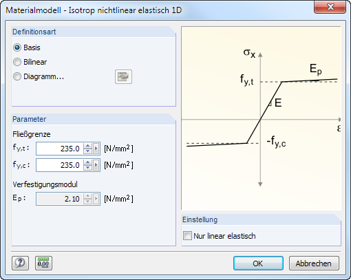
You have to define the yield strengths separately for tension (f_y,t) and compression (f_y,c) of the ideally or bilinearly elastic material. You can also define a stress-strain Diagram to display the material behavior realistically (see Figure 4.44).

If you have set the 3D model type (see Figure 12.23), you can define the plastic properties of the isotropic material in a dialog box. RFEM takes these properties for member elements into account, for example for the plastic calculation of a kinematic chain.

• Divide Member Using n Intermediate Nodes dialog box (see Figure 11.91), method of division: Place new nodes on the line without dividing it
• FE Mesh Settings dialog box (see Figure 7.10), option: Use division for straight members with a Minimum number of member divisions of 10

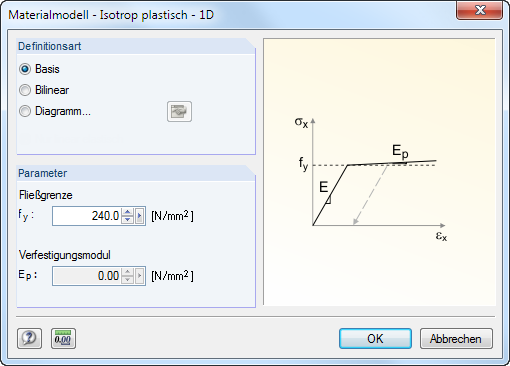
Define the parameters of the ideally or bilinearly plastic material. You can also define a stress-strain Diagram to display the material behavior realistically.

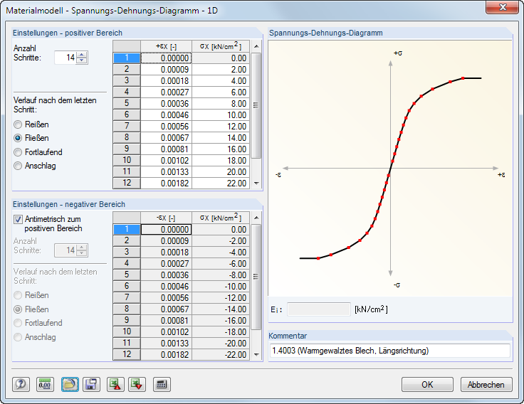
The material properties can be defined separately for the positive and the negative zone. The Number of steps determines the number of definition points respectively available. Enter the strains ε and the corresponding normal stresses σ into the two lists.

You have several options for the Diagram after last step: Tearing for material failure when exceeding a certain stress, Yielding for restricting the transfer of a maximum stress, Continuous as in the last step, or Stop for restricting to a maximum allowable deformation.

It is also possible to import parameters from an [Excel] worksheet.

Watch the dynamic graphic in the Stress-Strain Diagram dialog section to check the material properties. The dialog field E_i below the graphic shows the modulus of elasticity E for the current definition point.

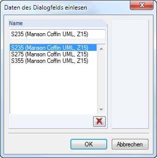
Use the button in the dialog box to save the stress-strain diagram so that you can apply it to different models. To import user-defined diagrams, click the button.

With this material model, you can display the properties of nonlinear materials for surfaces and solids. No energy is delivered to the model (conservative analysis). As the same stress-strain relations apply for loading and relief of load, no permanent plastic distortions are available after a relief.

You have to define the yield strengths f_y,t of the ideally or bilinearly elastic material. For the hypotheses according to von Mises and Tresca, they are equally applicable for tension and compression. For an authentic display of the material behavior, you can also define a stress-strain Diagram (see Figure 4.44).

The elasticity matrix is damped isotropically in order for the stress-strain relations of the equivalent stresses and distortions to be fulfilled.

Four calculation theories are available in the Strain Hypothesis dialog section:

• von Mises:

${\sigma }_{eqv}=\sqrt{{\sigma }_x^2+{\sigma }_y^2-{\sigma }_x{\sigma }_y+3{\tau }_{xy}^2}$

${\epsilon }_{eqv}=\frac{{\sigma }_{eqv}}{E}$

• Tresca

${\sigma }_{eqv}=\sqrt{{({\sigma }_x-{\sigma }_y)}^2+4{\tau }_{xy}^2}$

• Drucker-Prager:
• A criterion that tends to 1 is analyzed (in the plastic sense). Tension and compression stresses interact in the equations. During the evaluation, you should pay attention to the design ratio under the Criteria, not to the stresses.

• Mohr-Coulomb:
• Similar to the Drucker-Prager model, a stress circle is analyzed, though it is based on the Tresca hypothesis.

With the Only linearly elastic option, it is possible to deactivate the nonlinear material properties, for example for comparative analyses.

This material model shows an isotropic material behavior in the elastic zone. The plastic zone is based on the yielding according to different Strain Hypotheses with a user-defined Yield strength of the equivalent stress for surfaces and solids.

Specify the parameters of the ideally or bilinearly plastic material. You can also define a stress-strain Diagram to realistically display the material behavior (see Figure 4.44). According to von Mises and Tresca, the same yield strengths apply for tension and compression.

The yield conditions for 2D elements according to von Mises, for example, are mentioned in Equation 4.3. For 3D elements, they are as follows:

${\sigma }_{eqv}=\frac{1}{\sqrt{2}}\sqrt{({\sigma }_x-{\sigma }_y{)}^2+({\sigma }_y-{\sigma }_z{)}^2+({\sigma }_x-{\sigma }_z{)}^2+6({\tau }_{xy}^2+{\tau }_{xz}^2+{\tau }_{yz}^2)}$

In the elastic-plastic calculation, the total strain ε is divided into an elastic component ε_el and a plastic component ε_pl.

$\epsilon ={\epsilon }_{\mathrm{el}}+{\epsilon }_{\mathrm{pl}}$

However, this breakdown is only valid when assuming that the plastic strains are small (ε_pl < 0.1). If the plastic strains exceed this limit value, the plastic results should be evaluated with caution. This has to be taken into account in particular for calculations according to the large deformation analysis.

You can define stiffness properties that appear differently in both surface directions x and y. This way, you can model ribbed floors or stress directions of reinforced ceilings, for example. The surface axes x and y are perpendicular to each other in the surface plane (see Figure 4.75).

With this material model, you can globally assign an orthotropic property to all surfaces that consist of a particular material. Alternatively, it is possible to individually define the parameters for each surface (see Chapter 4.12).

An orthotropic elastic material is characterized by the moduli of elasticity E_x and E_y, the shear moduli G_yz, G_xz, and G_xy, as well as Poisson's ratio ν_xy and ν_yx. The elasticity matrix (inverse of stiffness matrix) is defined as follows:

$\left[\begin{array}{c}{\epsilon }_x\\ {\epsilon }_y\\ {\gamma }_{xy}\\ {\gamma }_{yz}\\ {\gamma }_{xz}\end{array}\right]=\left[\begin{array}{ccccc}\frac{1}{E_x}& -\frac{{\nu }_{yx}}{E_y}& 0& 0& 0\\ -\frac{{\nu }_{xy}}{E_x}& \frac{1}{E_y}& 0& 0& 0\\ 0& 0& \frac{1}{G_{xy}}& 0& 0\\ 0& 0& 0& \frac{1}{G_{yz}}& 0\\ 0& 0& 0& 0& \frac{1}{G_{xz}}\end{array}\right]·\left[\begin{array}{c}{\sigma }_x\\ {\sigma }_y\\ {\tau }_{xy}\\ {\tau }_{yz}\\ {\tau }_{xz}\end{array}\right]$

The following correlation exists between principal Poisson's ratio ν_xy and secondary Poisson's ratio ν_yx:

$\frac{{\nu }_{yx}}{E_y}=\frac{{\nu }_{xy}}{E_x}$

The following conditions must be met for a positively definite stiffness matrix:

• E_x > 0;     E_y > 0
• G_yz > 0;    G_xz > 0;    G_xy > 0

In a three-dimensional material model, you can define elastic stiffnesses separately in all directions of the solid. This way, you can display the strength properties of wood-based materials, for example.

The elasticity matrix is defined as follows:

$\left[\begin{array}{c}{\epsilon }_x\\ {\epsilon }_y\\ {\epsilon }_z\\ {\gamma }_{yz}\\ {\gamma }_{xz}\\ {\gamma }_{xy}\end{array}\right]=\left[\begin{array}{cccccc}\frac{1}{E_x}& -\frac{{\nu }_{yx}}{E_y}& -\frac{{\nu }_{zx}}{E_z}& 0& 0& 0\\ -\frac{{\nu }_{xy}}{E_x}& \frac{1}{E_y}& -\frac{{\nu }_{zy}}{E_z}& 0& 0& 0\\ -\frac{{\nu }_{xz}}{E_x}& -\frac{{\nu }_{yz}}{E_y}& \frac{1}{E_z}& 0& 0& 0\\ 0& 0& 0& \frac{1}{G_{yz}}& 0& 0\\ 0& 0& 0& 0& \frac{1}{G_{xz}}& 0\\ 0& 0& 0& 0& 0& \frac{1}{G_{xy}}\end{array}\right]·\left[\begin{array}{c}{\sigma }_x\\ {\sigma }_y\\ {\sigma }_z\\ {\tau }_{yz}\\ {\tau }_{xz}\\ {\tau }_{xy}\end{array}\right]$

The following correlations exist between principal Poisson's ratios ν_yz, ν_xz, ν_xy and secondary Poisson's ratios ν_zy, ν_zx, ν_yx:

$\frac{{\nu }_{zy}}{E_z}=\frac{{\nu }_{yz}}{E_y}; \frac{{\nu }_{zx}}{E_z}=\frac{{\nu }_{xz}}{E_x}; \frac{{\nu }_{yx}}{E_y}=\frac{{\nu }_{xy}}{E_x}$

The following conditions must be met for a positively definite stiffness matrix:

• E_x > 0;      E_y > 0;      E_z > 0
• G_yz > 0;    G_xz > 0;    G_xy > 0

The material model according to Tsai-Wu unifies plastic with orthotropic properties. This way, you can enter special modelings of materials with anisotropic characteristics such as plastics or timber. When the material is yielding, stresses remain constant. A redistribution is carried out according to the stiffnesses available in the individual directions.

The elastic zone corresponds to the Orthotropic Elastic - 3D material model (see above). For the plastic zone, the yielding according to Tsai-Wu applies:

$f_{\text{crit}}\left(\sigma \right)=\frac{1}{C}\left[\frac{({\sigma }_x-{\sigma }_{x,0}{)}^2}{f_{t,x}{f}_{c,x}}+\frac{({\sigma }_y-{\sigma }_{y,0}{)}^2}{f_{t,y}{f}_{c,y}}+\frac{({\sigma }_z-{\sigma }_{z,0}{)}^2}{f_{t,z}{f}_{c,z}}+\frac{{\tau }_{yz}^2}{f_{v,yz}^2}+\frac{{\tau }_{xz}^2}{f_{v,xz}^2}+\frac{{\tau }_{xy}^2}{f_{v,xy}^2}\right]$

where

${\sigma }_{x,0}=\frac{f_{t,x}-f_{c,x}}{2}$

${\sigma }_{y,0}=\frac{f_{t,y}-f_{c,y}}{2}$

${\sigma }_{z,0}=\frac{f_{t,z}-f_{c,z}}{2}$

$C=1+{\left[\frac{1}{f_{t,x}}+\frac{1}{f_{c,x}}\right]}^2\frac{E_x{E}_{p,x}}{E_x-E_{p,x}}\alpha +\frac{{\sigma }_{x,0}^2}{f_{t,x} f_{c,x}}+\frac{{\sigma }_{y,0}^2}{f_{t,y }{f}_{c,y}}+\frac{{\sigma }_{z,0}^2}{f_{t,z} f_{c,z}}$

f_t,x, f_t,y, f_t,z : Plastic ultimate tensile strength in direction x, y, or z
f_c,x, f_c,y, f_c,z : Plastic ultimate compressive strength in direction x, y, or z
f_v,yz, f_v,xz, f_v,xy : Plastic shear strength in direction yz, xz, or xy
E_p,x : Hardening modulus
α : State variable of hardening

$\alpha =\sum _i\Delta {\gamma }_i$

All strengths must be defined positively.

The stress criterion can be imagined as an elliptical surface within a six-dimensional space of stresses. If one of the three stress components is applied as a constant value, the surface can be projected onto a three-dimensional stress space (see Figure 4.51).

If the value for f_y(σ) as per Equation 4.12 is lower than 1, stresses lie in the elastic zone. The plastic zone is reached as soon as f_y(σ) = 1. Values higher than 1 are not allowed. The model behavior is ideal-plastic, which means no stiffening takes place.

With this elastoplastic material model you can consider material softening, which can be different in the local x- and y-direction of the surface. The material model is suitable for unreinforced masonry walls with in-plane loads. The total strain tensor ε is divided into the sum of its elastic and plastic components (ε = ε_el + ε_pl). This approach is based on the assumption that the damage represents a "smeared" crack behavior in which the material is a continuum even after the damage.

In addition to the material properties of an orthotropic elastic 2D material model, the dialog box includes seven strength parameters (f_t,x, f_t,y, f_c,x, f_c,y, α, β, γ) and five parameters for describing the inelastic behavior (G_t,x, G_t,y, G_c,x, G_c,y, κ_p). These parameters can be determined in experimental setups where single and biaxial compression and tension loads are analyzed. The correlation coefficients are as follows:

$\alpha =\frac{1}{9}\left(1+4\frac{f_{t,x}}{f_{\alpha }}\right)\left(1+4\frac{f_{t,y}}{f_{\alpha }}\right)$

$\beta =\left(\frac{1}{f_{\beta }^2}-\frac{1}{f_{c,x}^2}-\frac{1}{f_{c,y}^2}\right)f_{c,x} f_{c,y}$

$\gamma =\left[\frac{16}{f_{\gamma }^2}-9\left(\frac{1}{f_{c,x}^2}+\frac{\beta }{f_{c,x} f_{c,y}}+\frac{1}{f_{c,y}^2}\right)\right]f_{c,x} f_{c,y}$

For the tension range, uses a hypothesis according to Rankine, while a yield criterion according to Hill is used for the pressure range. In the equations above, the parameter α describes the proportion of the shear stresses that lead to failure under tensile stress. In the case of compression, the shear component is analogously expressed by the parameters β and γ.

The following figure shows a typical yield surface for the anisotropic Rankine-Hill failure criterion.

Temperature-dependent stress-strain properties of an elastic isotropic material can be defined in a diagram or imported from [Excel]. These properties are considered for member and surface elements subjected to thermal load (changes or differences in temperature).

The Reference temperature defines stiffnesses for the members or surfaces that have no temperature loads. For example, if a reference temperature of 300 °C is set, the reduced elastic modulus of this point of the temperature curve is applied to all members and surfaces.

The Options dialog section allows you to control if the Poisson's ratios that are applied to the complete temperature diagram are identical. Clear the check box to access the Poisson's Ratio table column for individual entries.

Use the [Load] button to import predefined temperature diagrams for different steel alloys (see Figure 4.45).

Click the [Save] button to save user-defined temperature diagrams so that you can use them for other models.

Use this material model to consider masonry walls not able to bear tension forces and reacting with formation of cracks.

The dialog box allows you to define the Limit tension stresses in direction of the surface axes x and y, which means parallel and perpendicular to the support interstices. In several iterations during calculation, RFEM then finds out, which finite elements become stress-free due to the failure criterion.

If numerical problems occur during calculation, you can try to reach convergence by increasing the Hardening factor C_H.

If the masonry material has already been defined in the library before you open the Material Model dialog box, the following limit values are preset:

Table 4.1 Limit tension stresses according to masonry standards

Standard	σx,limit	σy,limit
DIN 1053-100	fx2 Tensile strength parallel to interstice of support	0
EN 1996-1-1	fxk1 Tensile strength parallel to interstice of support	fxk2 Tensile strength perpendicular to interstice of support

With this material model, you can model the material behavior of steel fiber concrete where a continuous reduction of strength occurs due to cracking.

The stress-strain curve of the steel fiber concrete is defined in a Diagram that can be accessed with the button. This diagram is shown in Figure 4.44.

In this material model ("Mazars' damage model"), the isotropic stiffness is reduced with a scalar damage parameter. This damage parameter is determined from the stress curve defined in the Diagram. The direction of the principal stresses is not taken into account. Rather, the damage occurs in the direction of the equivalent strain, which also covers the third direction perpendicular to the plane. The tension and compression area of the stress tensor is treated separately. Different damage parameters apply in each case.

The Reference element size controls how the strain in the crack area is scaled to the length of the element. With the default value zero, no scaling is performed. Thus, the material behavior of the steel fiber concrete is modeled realistically.

The properties of many materials are stored in a comprehensive, expandable database.

To access the library, click the [Material Library] button (see Figure 4.40) in the New Material dialog box. You can also open the database in Table 1.3 Materials (see Figure 4.41): Place the cursor into table column A and click the button shown on the left or use the [F7] key on the keyboard.

Select a material from the Material to Select list and check the corresponding parameters in the lower part of the dialog box. Click [OK] or [↵] to carry it over to the previous dialog box or the table.

As the material library is very large, there are various selection options available in the Filter dialog section. You can filter the material list according to Material category group, Material category, Standard group, Standard, and Special application. This way, you can reduce the provided data.

With the Include invalid check box, you can select if materials of "old" standards are also displayed in the library.

With the and buttons, you can create and edit categories.

To adjust the sequence of the items, use the and buttons.

Often, the use of a few materials is already sufficient for daily engineering work. You can mark these materials as your favorites. Use the [Create New Favorites Group] button to open the dialog box for defining preferred materials.

Enter the Name of the new favorites group. After clicking [OK], a new dialog box appears which is structured like the material library. The filter options described above are also available in this dialog box.

In the Material Library - Favorites dialog section, you can mark your preferred materials by selecting their check boxes. To change the sequence of materials, use the and buttons.

After closing the dialog box, the material library presents a clear overview of favorites as soon as you activate the Favorites group option and the group is specified in the list.

The material library can be extended. If you add a new material, you can use it for all available models.

Click the button in the library (to the left of the Search field, see Figure 4.60). The New Material dialog box opens. The parameters of the entry selected in the Material to Select list are preset. Creating a new material is easier when you choose a material with similar properties first.

Enter the Material Description, define the Material Properties, and assign the material to the appropriate groups and categories for Filter functions.

If you use custom materials, you should save the Materialien_User.dbd file before installing an update. The file can be found in the master data folder of RFEM 5 C:\ProgramData\Dlubal\RFEM 5.xx\General Data.