


A static analysis setting (SA) specifies the rules according to which load cases and load combinations are calculated. Three standard analysis types are preset.
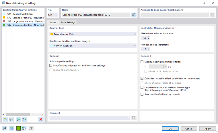
Main
The Main tab manages the settings for the structural analysis and elementary calculation parameters.
Analysis Type
This dialog section controls the calculation theory according to which load cases and load combinations are analyzed. In the "Analysis Type" list, three approaches are available for selection.
Geometrically linear
When calculating according to the geometrically linear analysis (first-order), the equilibrium is analyzed on an undeformed structural system. A linear analysis is carried out because deformations of the components are not included in the calculation.
Load cases are calculated according to the geometrically linear analysis by default.
Second-order (P-Δ)
In the "structural" second-order analysis, the equilibrium is determined on a deformed structural system. Deformations are assumed to be small. Axial forces in the system have an impact on an increase in bending moments. Thus, this analysis comes into effect when axial forces are significantly greater than shear forces.
Load combinations are calculated nonlinearly by default according to the second-order analysis.
Large deformations
The large deformation analysis (third-order or theory of large deformations) considers longitudinal and transversal forces in the calculation. After each iteration step, the stiffness matrix of a deformed system is created. The loads keep their originally defined direction of action when the members are twisted.
If the model includes cable members, the calculation according to the large deformation analysis is preset.
Iterative Method for Nonlinear Analysis
For solving the nonlinear algebraic system of equations according to second-order and large deformation analysis, the Newton-Raphson method is used.
Newton-Raphson
The nonlinear equation system is solved numerically by means of iterative approximations with tangents. The tangential stiffness matrix is determined as a function of the current state of deformation; it is inverted in each cycle of iterations. In the majority of cases, a fast (quadratic) convergence is reached.
Newton-Raphson with postcritical analysis
For solving problems of postcritical analysis according to the large deformation analysis, a certain instability has to be overcome. If an instability is available and the stiffness matrix cannot be inverted, the stiffness matrix of the last stable iteration step is used. This matrix is used for further calculations until the stability range is reached again.
Controls for Nonlinear Analysis
The "Maximum number of iterations" defines the highest number of calculation runs for an analysis according to the second-order or large deformation analysis, as well as for non-linearly acting objects. When the calculation reaches the limit without reaching an equilibrium, a corresponding message appears. Then, you can decide if you want to display the results.
The "Number of load increments" is relevant for calculations according to second-order or large deformation analysis. When considering large deformations, it is often difficult to find an equilibrium. Instabilities can be avoided by applying loading in several steps. For example, if you specify two load increments, half of the load is applied in the first step. It is iterated until the equilibrium is found. Then, in the second step, full loading is applied to the already deformed system and iterations are run again until the equilibrium is reached.
Options I
In this dialog section, you can activate various "special settings" to manipulate calculations according to the second-order or large deformation analysis.
Modify standard precision and tolerance settings
When you select the "Modify standard precision and tolerance settings" check box, the Precision and Tolerance tab is added to the dialog box. There, you can adjust the convergence criteria.
Ignore all nonlinearities
With the "Ignore all nonlinearities" check box, you can deactivate the nonlinear properties of elements for the calculation. Tension members, for example, remain in the model whenever compressive forces occur. However, you should suppress the non-linear properties only for test purposes; for example, to find the cause of an instability. Incorrectly defined failure criteria are sometimes responsible for calculation break-offs.
Options II
Modify loading by multiplication factor
After selecting the check box, you can define a factor k by which all loads are to be multiplied.
Older standards claim to multiply loads globally by a certain factor in order to increase effects according to the second-order analysis for stability design checks. In turn, the design must be carried out with the service loads. Both requirements can be met by entering a factor greater than 1 and activating the "Divide results by load factor" check box.
For analyses according to current standards, the loading should not be edited by means of factors. Instead, the partial safety and combination factors are to be taken into account for the superposition in the design situations.
Consider favorable effect due to tension in members
Tensile forces have a favorable effect on pre-deformed structural systems. Thus, the deformation is reduced and the structure is stabilized. Usually, we benefit from this effect in calculations according to the second-order and large deformation analysis; for example, for halls with bracings or general structures subjected to bending. Relief due to tension force effects for beams trussed from below (beams with supporting ties or cables) may result in an unwanted reduction of deformations and internal forces.
Displacements due to member load of "Pipe internal pressure" type
The check box is relevant for the member load called pipe internal pressure. The Bourdon effect describes the effort of a bent pipe to straighten under the influence of pressure. Both perimeter stresses and axial stresses caused by internal pressure load lead to longitudinal strain of the pipe, considering material stiffness and transversal strain.
See this technical article describing an example of how the internal pressure of pipes is calculated.
Save results of all load increments
If the loading is applied incrementally (see Controls for Nonlinear Analysis), you can use this check box to force the output of intermediate results in order to check the results of the individual load increments.
Basic Settings
The Basic Settings tab manages the basic specifications for the calculation.
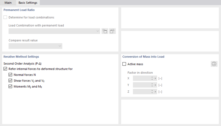
Permanent Load Ratio
The "Determine for load combinations" check box offers the possibility to determine the ratio of a permanently acting load in a load combination. Select the load combination in the list, or create a new load combination with the
![]() button. Then, in the "Compare result value" list, you can define the ratios that have a static or variable effect.
button. Then, in the "Compare result value" list, you can define the ratios that have a static or variable effect.
The ratio of the permanent load can be considered as conforming to the standards in the design.
Iterative Method Settings
The check boxes in this dialog section are important for the "Second-order (P-Δ)" analysis.
Refer internal forces to deformed structure
The internal forces of members are usually output in relation to the modified position of the member coordinate systems that is present in the deformed system. If you want the output to refer to the undeformed initial system, you can define the relevant member internal forces and moments by deactivating the corresponding check boxes.
Conversion of Mass into Load
Loads can be defined not only as forces and moments, but also in the form of masses. However, masses have no effect in the structural analysis. If you want to consider them, select the "Active mass" check box. Then, enter the "Factor in direction" to describe the effect of the mass. Thus, the masses are converted into forces before the calculation starts, and they are included in the determination of internal forces and moments.
Use the
![]() button to switch between entering the mass factor and entering the acceleration directly. The name of the input fields is adjusted accordingly.
button to switch between entering the mass factor and entering the acceleration directly. The name of the input fields is adjusted accordingly.
Precision and Tolerance
The Precision and Tolerance tab allows you to influence the convergence parameters of the calculation. However, you should change the default settings only in exceptional cases.
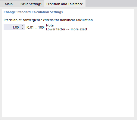
Precision of convergence criteria of nonlinear calculation
If non-linear effects are acting, or if the second-order or large deformation analysis is performed, the calculation can be influenced by means of convergence criteria.
The change of axial forces in the last two iterations is compared member by member. As soon as this change reaches a specific fractional amount of the maximum axial force, the calculation stops. However, during the iterations it may happen that the axial forces oscillate between two values. You can prevent this pendulum effect by adjusting the "sensitivity".
The precision also affects the convergence criterion for deformation changes in calculations performed according to the large deformation analysis, where geometric non-linearities are considered. The default value is 1.00. The minimum factor is 0.01, the maximum value 100.00. The smaller the value is, the closer the convergence term must be to the comparison term. The result accuracy is increased accordingly.