Introduction
The finite element method is used whenever mechanical problems cannot be solved analytically. Often, nonlinear effects such as failure under pressure (geometric nonlinearity), plastic yielding (material nonlinearity), and contact or kinematic degrees of freedom are also taken into account. These effects, especially for nonlinear material models, can be considered by using an iterative calculation method.
FEM Setting
Basic steps for FEM setting (further information can be found in [1]):
- Weak form of equilibrium
δu
Virtuelle (Test-)Verschiebung
t0
Anfangslastfaktor
σdV
Innere Kräfte
ρbdV
Volumenkräfte
B
integriertes Gebiet
- Conversion to Voigt notation with Tensor 4 Step
C
Steifigkeitsmatrix
δε
Variation des Verzerrungszustands
B
integriertes Gebiet
ε
Dehnung
u
Verformung
- This notation is used in the following text to solve the approximate solution of the FE approach for nonlinear materials.
- For this, the displacement field is multiplied by the approach functions.
u(x,t)
Verschiebung über Zeit (Lastinkrement)
H
Formfunktion
û
Knotenverschiebung
Inserting the derivative of displacement into the weak form. Numerical integration is used to calculate the nodal displacement, stresses, and strains in post-processing by means of the material rule.
Newton-Raphson Iteration Sequence
Due to the nonlinear material behavior, the material matrix C in Equation 2 above changes with each expansion step. The standard calculation method for solving this problem is the Newton-Raphson iteration. It is used to linearize the function in a starting point. The stiffness matrix C of the preliminary step is always used in the iteration. In the linearized iteration step, a tangent is placed at the zero of the function.
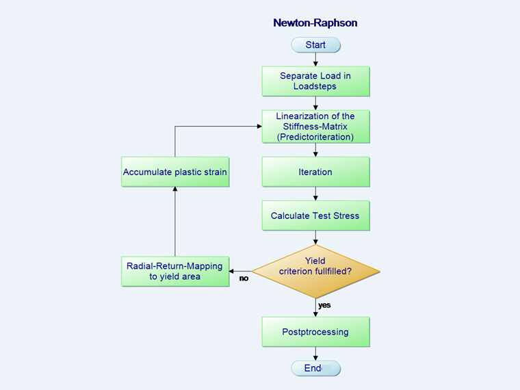
The equations belonging to the flowchart in the image above are the following:
- Dividing the load into load steps.
- Predictor Step
K
Steifigkeitsmatrix des vorherigen Zeitschritts
t+Δtfext
Äußere Kräfte um eine weitere Laststufe erhöht
0tfint
Innere Kräfte des vorherigen Zeitschritts
ϕ
Verzerrung
- In Point 3, iteration of the flowchart, the total distortion reduced by the plastic distortion is calculated (corrector step). The objective of the iterative calculation is always that the sum of the loads is zero. However, this is impossible numerically. Therefore, a break-off limit ε is defined at which the calculation is interrupted as sufficiently accurate.
R
Abbruchrate
fext
äußere Kräfte
fint
innere Kräfte
ε
Epsilon Abbruchrate
t
Zeitschritt
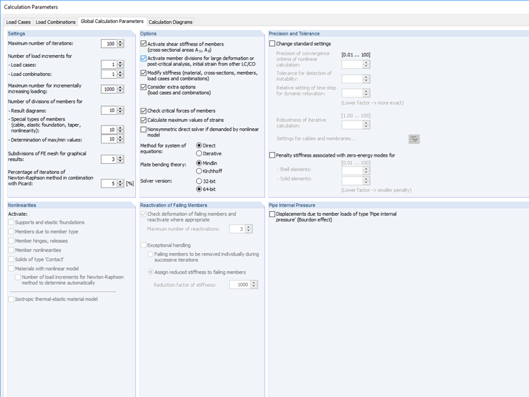
In the program, the break-off limit can be set among the calculation parameters.
The following image shows the flow of a Newton-Raphson iteration. In the first iteration
the break-off R or ε is not reached. The tolerance limit is not reached in the second iteration (red) either. Only in the third iteration is the distance of the tangent stiffness so small that convergence is achieved.
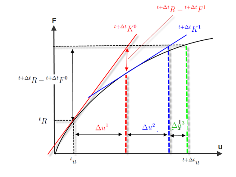
As already mentioned, the deformation is continuously summed up during the iteration.
Conclusion
The Newton-Raphson iteration has the consistency or convergence order 2. The number of "correct" locations in the iteration doubles with each step. Thus, a Newton-Raphson iteration converges quadratically, and the accuracy increases with each iteration when the method converges. However, if the method does not converge, the error goes to infinity and the calculation is stopped.
Error causes are, for example, a slope of the load-deformation curve that is too steep, and a curve gradient in the plastic area that is too flat. If the load-deformation curve in the image above showed a break in the second iteration step that was too strong, the material tangent and thus the stiffness matrix would not correctly display the slope of the elastic area. In this case, the slope of the root would be wrong for the plastic area. This is one of the reasons that an increase in the load steps is accompanied by an improved convergence.