A modal analysis setting (MOS) specifies the rules according to which eigenvalues are calculated. Two standard analysis types are preset. You can adjust these types or create further modal analysis settings at any time.
Main
The Main tab manages the settings required for the modal analysis, as well as some other elementary calculation parameters. RFEM and RSTAB provide different options for selecting the eigenvalue method.
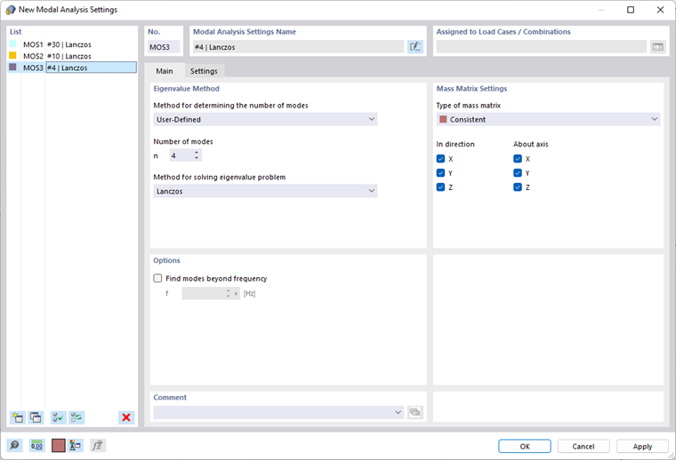
Eigenvalue Method
In this section, you can define which method is used to analyze the eigenvalue problem and how many mode shapes are determined.
Method for determining the number of modes
You can select from three options in the list.
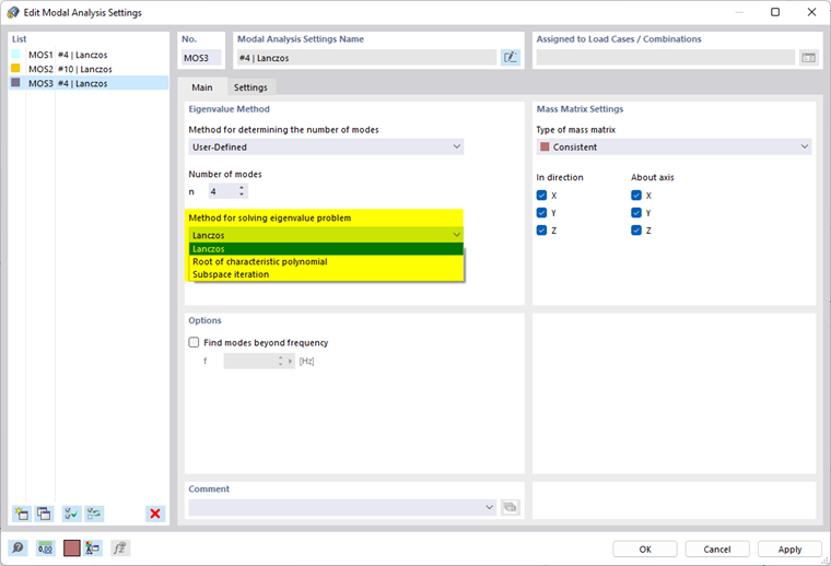
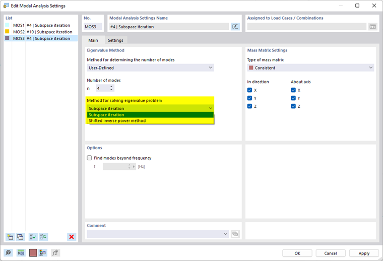
- User-defined
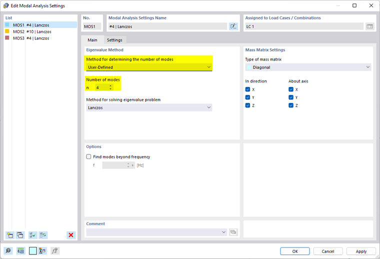
The user-defined method allows you to specify the number of the smallest modes to be calculated. It is possible to define up to 9,999 mode shapes. In addition to this limit, the model also represents a restriction on the number of possible mode shapes: It corresponds to the degrees of freedom that result from the number of free mass points multiplied by the number of the directions in which the masses act.
- Automatic, to reach effective modal mass factors
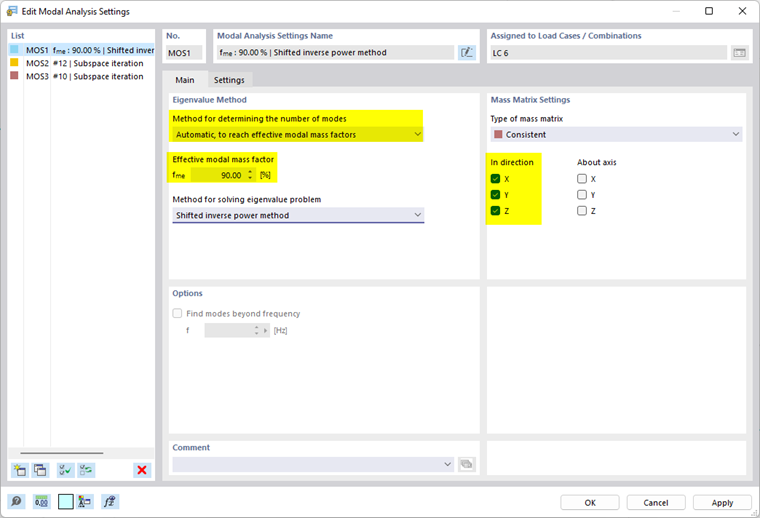
The program determines as many mode shapes as necessary until the specified modal mass factor is reached. The effective modal mass factors are analyzed for the specified translational directions (X, Y, Z).
- Automatic, to reach maximum natural frequency
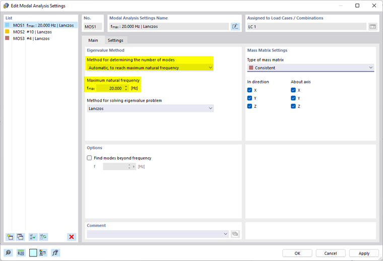
The program determines as many mode shapes as necessary until the specified natural frequency is reached.
Method for solving eigenvalue problem (for RFEM)
In the list, three methods are available to solve the eigenvalue problem. If you have set the automatic method for determining the number of eigenvalues, only one solving method is available.
For more information about the individual methods, see Bathe [1] and Natke [2].
- Lanczos
The Lanczos method is suitable as an iterative method for determining the lowest eigenvalues and the corresponding mode shapes of large models. In most cases, this algorithm allows reaching a quick convergence. It is possible to calculate up to n–1 mode shapes (n: degrees of freedom of the model with mass).
An introductory description can be found at en.wikipedia.org/wiki/Lanczos_algorithm.
- Root of characteristic polynomial
With this method, the analytical solution of an eigenvalue problem is carried out in a direct method. The main advantage of this method is the precision of higher eigenvalues and the fact that all the eigenvalues of the model can be determined. For larger models, this method may be quite time-consuming.
An introductory description can be found at en.wikipedia.org/wiki/Characteristic_polynomial.
- Subspace iteration
Using this method, all eigenvalues are determined in one step. In this case, the spectrum of the stiffness matrix has a strong influence on the duration of the calculation. Therefore, this method is only recommended for large FE models if you want to calculate a few eigenvalues. The working memory limits the number of eigenvalues that can be determined in a reasonable amount of time.
An introductory description can be found at en.wikipedia.org/wiki/Krylov_subspace.
Method for solving eigenvalue problem (for RSTAB)
In the list, two methods are available to solve the eigenvalue problem. If you have specified one of the automatic methods for determining the number of eigenvalues, only one solving method is available.
For more information about the individual methods, see Bathe [1].
- Subspace iteration
Using this method, all eigenvalues are determined in one step. In this case, the spectrum of the stiffness matrix has a strong influence on the duration of the calculation. Therefore, this method is only recommended for large FE models if you want to calculate a few eigenvalues. The working memory limits the number of eigenvalues that can be determined in a reasonable amount of time.
An introductory description can be found at en.wikipedia.org/wiki/Krylov_subspace.
- Shifted inverse power method
This method is based on assumptions for the eigenvectors of the mode shapes, which are iteratively approximated to a convergent solution during the calculation. The advantage of this method is the short calculation time due to the rapid convergence. "Shift" means that this method can also be used to determine all results between the largest and the smallest eigenvalues of the given matrix.
An introductory description can be found at en.wikipedia.org/wiki/Inverse_iteration.
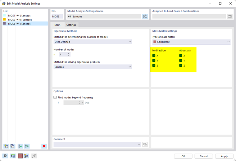
Mass Matrix Settings
In this dialog section, you can define which mass matrix is used and in or about which axes the masses should act in the modal analysis.
Type of Mass Matrix
Three types of mass matrices are available for selection in the list.
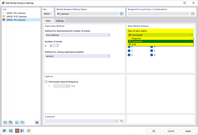
- Diagonal
In the case of the diagonal mass matrix M, the masses are assumed to be concentrated on FE nodes. The input in the matrix is the concentrated masses in the translational directions X, Y and Z, as well as the rotational directions about the global axes X (φX), Y (φY), and Z (φZ). It is necessary to distinguish the following two cases:
– Diagonal matrix with only translational degrees of freedom: If only the translational directions are activated for the diagonal matrix, the diagonal matrix results in:
– Diagonal matrix with translational and rotational degrees of freedom: If the translational directions as well as the rotational directions are activated, the diagonal matrix results in:
|
m |
Mass |
|
IX, IY, IZ |
Mass moments of inertia (RFEM 6) |
- Consistent
The consistent mass matrix is a complete mass matrix of finite elements. Therefore, the masses are not concentrated on the FE node. Instead, the shape functions are used for a more realistic distribution of masses within the finite elements. Using this mass matrix, non-diagonal entries in the matrix are considered, so that rotation of the masses is generally taken into account. The consistent mass matrix is structured as follows (the shape functions are neglected for the sake of simplicity):
- Unit
The unit matrix overwrites all previously defined masses. This matrix is a consistent matrix where all diagonal elements are 1 kg. The mass is set to 1 at each FE node. Translations and rotations of masses are taken into account. This mathematical approach should be used for numerical analyses only.
More information on matrix types and especially on the use of the unit matrix can be found in Barth/Rustler [3].
In direction / About axis
Six check boxes control in which direction or about which axes the masses act when determining the eigenvalues. The masses can act in the global displacement directions X, Y, or Z, and rotate about the X, Y, and Z axes. Select the relevant check boxes. It is necessary to activate at least one direction or axis in order to calculate the eigenvalues.
Options
The last dialog section in the "Main" tab provides an important setting option for the modal analysis.
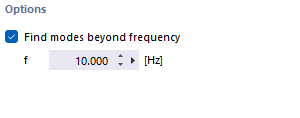
Find modes beyond frequency
If individual members or surfaces in the model have a very low natural frequency, they occur as local mode shapes first. If you select the check box, only the eigenvalues above a certain value "f" of the natural frequency will be calculated. In this way, you can reduce the number of results and limit it to the eigenvalues that are relevant to the global model.
Settings
The Settings tab manages further settings required for the modal analysis, as well as the elementary calculation parameters.
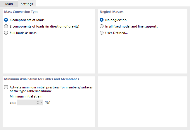
Mass Conversion Type
This dialog section controls the import of masses for the modal analysis. By default, only the "'Z-components of loads" are taken into account. This refers to the load components acting in both directions of the Z-axis – positive and negative.
With the "Z load components (in direction of gravity)" option, the program only applies the load components that are effective in the direction of gravity. The gravity is determined by the orientation of the global Z-axis (see the chapter Axis Orientation of the RFEM manual): It acts in the direction of the global Z-axis if it is oriented downwards. If the global Z-axis is oriented upwards, it has the opposite effect
Select the "Full loads as mass" option to import all loads and apply all components as masses.
Neglect Masses
The modal analysis takes into account all the masses defined in a model. This dialog section includes the option to neglect the mass of the model parts, such as the mass in all fixed nodal and line supports. You can also make a user-defined object selection.
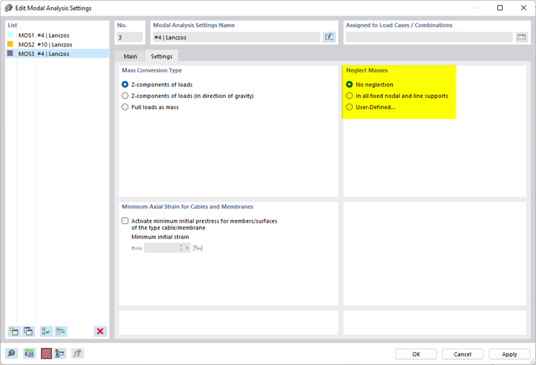
When selecting the "User-defined" option, the additional "Neglect Masses" tab appears. You can specify the objects without masses here.
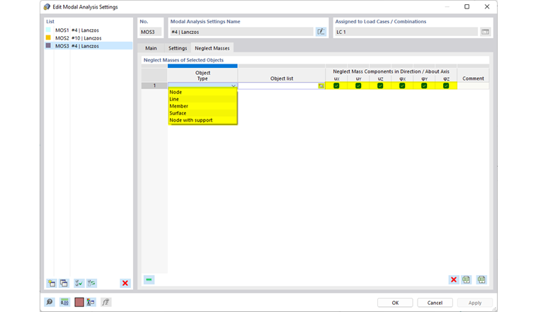
You can directly create the list of objects (nodes, lines, members, and so on) using the object numbers. As an alternative, use the
![]() button in the text box of the "Object List" to select the objects graphically. Click the
button in the text box of the "Object List" to select the objects graphically. Click the
![]() button to preset fixed supports only.
button to preset fixed supports only.
Use the check boxes for the displacement directions uX, uY, and uZ, as well as the rotations φX, φY, and φZ to define in which direction the masses are to be neglected.
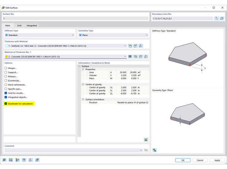
The stiffness of the objects whose masses are neglected is nevertheless considered in the matrix. If you also want to neglect the stiffness of these objects, you can use the Structure Modification to adjust the stiffnesses individually. It is also possible to deactivate the objects for the calculation (see the chapter of the RFEM manual).
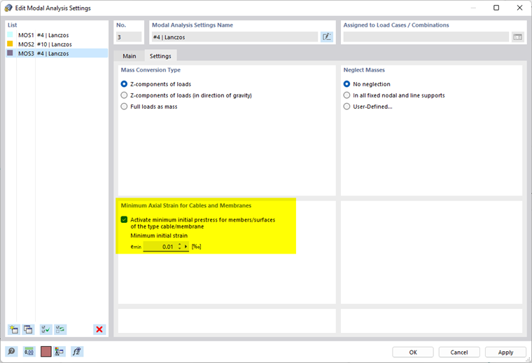
Minimum Axial Strain for Cables and Membranes
The correct entry of cable members and 6/000040#membrane membrane surfaces requires a minimum change in length. If the limit is set too low, the eigenvalues reached are not realistic and only local mode shapes are determined. The default value of the initial prestress for emin is suitable in most cases.