


The Main tab manages the specifications for the method and the time steps.
Time History Analysis Method Type
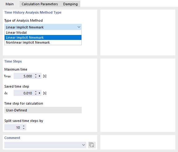
In the RFEM program, two linear and nonlinear analysis methods are available for selection in the list in this dialog section (see the image Defining Analysis Method and Time Steps):
- Linear Modal
- Linear Implicit Newmark
- Nonlinear Implicit Newmark
In RSTAB, the list contains two linear and two nonlinear analysis methods:
- Linear Modal
- Linear Implicit Newmark
- Nonlinear Explicit | Linear Static
- Nonlinear Explicit | Large Deformation
The first two analysis methods are geometrically linear, so they are only valid for small deformations. Furthermore, all nonlinear properties of the model are either ignored (for example, the failure of a support is not considered) or replaced (a tension member is represented by a truss).
The linear modal analysis method uses a decoupled system that is based on the model's eigenvalues and mode shapes, and is determined in the assigned Modal Analysis Load Case . The multi-degree-of-freedom system ("MDOF") is split into many single-degree-of-freedom systems ("SDOF") (diagonalized mass and stiffness matrix). A certain number of eigenvalues is required to ensure accuracy. The solution of the decoupled system is then determined with an implicit Newmark solver. The mass matrix settings and stiffness modifications are taken from the assigned modal analysis load case. If the eigenvalues have already been determined, this analysis method is slightly faster than the linear implicit Newmark analysis.
The linear implicit Newmark analysis is a direct time integration method. It requires sufficiently small time steps to achieve precise results. No natural vibration analysis is required for this analysis method. The theoretical background is explained in [1], for example. Using implicit solution methods, unknown values at time i + 1 are determined on the basis of the values at time i and i + 1. It is necessary to solve nonlinear equations; no iteration and convergence checks are required.
The nonlinear implicit Newmark analysis takes into account geometric and structural nonlinearities of the model. The method is unconditionally stable: There is no upper stability limit at the time step 𝛥t. Nevertheless, sufficiently small time increments are required for exact results. The time increment depends on the excitation, the frequency of the model and the complexity of the nonlinearities. There are no restrictions regarding the mass matrix and Rayleigh damping.
The nonlinear explicit method of RSTAB uses the method of central differences. It is suitable for excitations of short duration and rapidly changing nonlinearities in the model. The method is explicit, because unknown values are only based on time i and not on the unknown response at time i + 1. The explicit integration rule works well in combination with a diagonal mass matrix and with the constraint of the damping matrix '''C''' = '''αM'''. The method is conditionally stable: A limited solution is only achieved if the time increment Δt is smaller than the stable time increment Δtstable. The stability limit can be defined from the largest eigenvalue in the model ωmax and the component of the critical damping D in the largest mode shape.
In practice, the stable time increment can be determined using the following estimated value:
The dilatation wave velocity is determined for a linear elastic material (with Poisson's ratio equal to zero) from:
This estimated value allows for smaller time steps compared to the exact stability limit. With this estimation, however, it should be noted that many effects are not included and a smaller time step Δt may also be required for accuracy reasons. The program uses a fixed time step—the stable initial time increment or a user-defined value.
Time Steps
Enter the "Maximum time" tmax to be analyzed in the calculation. In the "Saved time step" text box, specify the interval Δt where the results should be saved. Results will only be available for these time steps. The dynamic envelope is also generated from the saved time steps.
In addition to the time steps saved, it is necessary to define time steps for the actual calculation. To do this, enter a value in the "Split saved time steps by" text box that should divide the saved time steps Δt.
For a successful time history analysis, you need to select the time steps "appropriately". In essence, the decision represents a compromise between calculation time and accuracy. The following recommendation can be made for the linear time history analysis (see [2]):
- Taking into account the accelerogram and the transient time diagrams, the shortest length of the discrete excitation should be divided into at least seven time steps.
- To calculate the time step, the highest frequency f of the model that is relevant for the system response should be used as follows: Δt ≤ 1 / (20f). Similarly, you should check whether the highest frequency of the excitation is covered in the condition Δt ≤ 𝜋 / (10ω). If not, it is necessary to adjust the time step.
